
Biostatistics — MCQs

On this page
A study is conducted to compare the mean hemoglobin (Hb) levels between two independent groups. Which statistical test is most appropriate?
In a village of 100 children, 10 children have a past history of measles (i.e., they are not at risk now), 20 new cases of measles were reported this year. What is the incidence of measles in this population for the year?
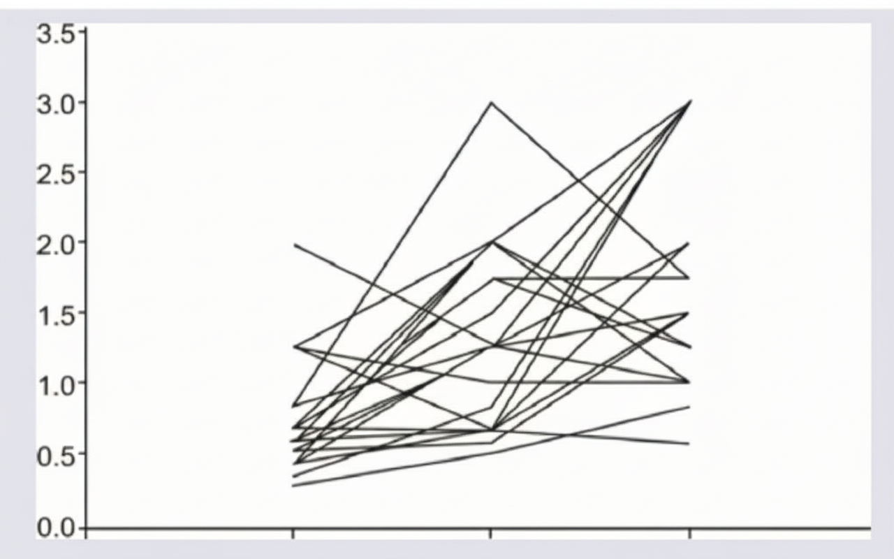
The given image shows:
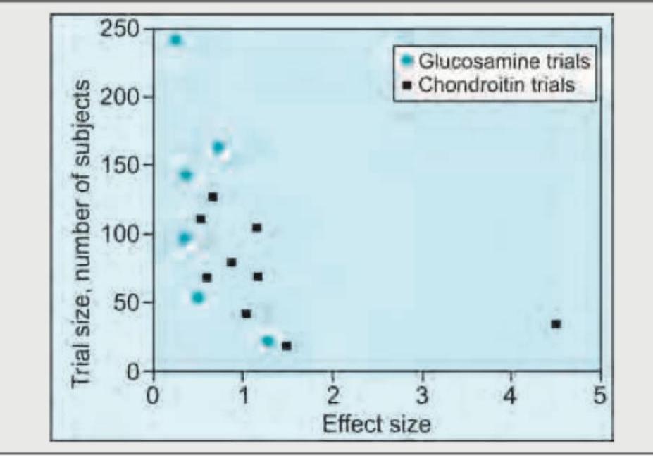
The given image shows:
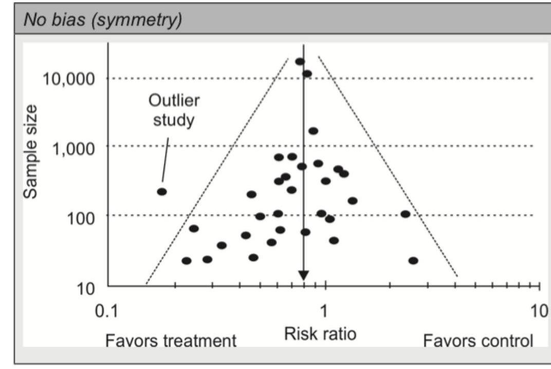
The given image shows:
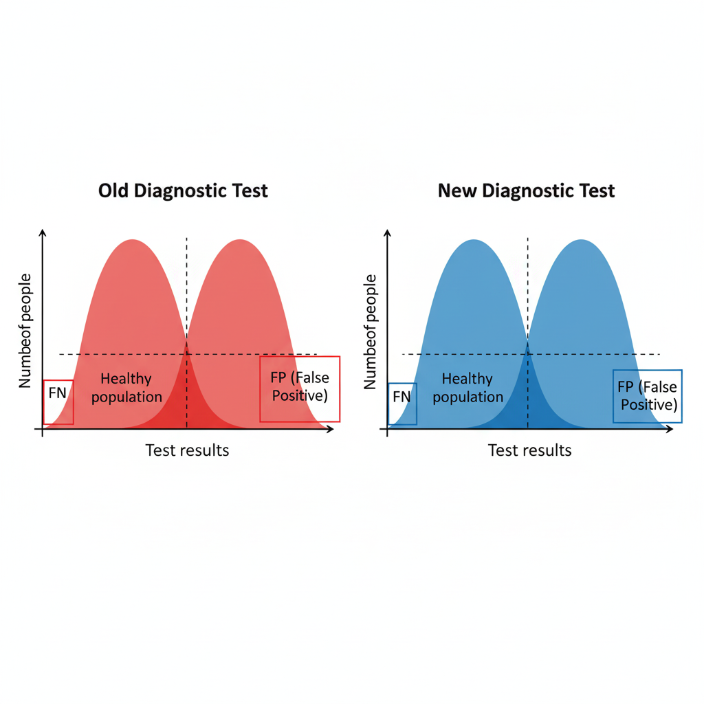
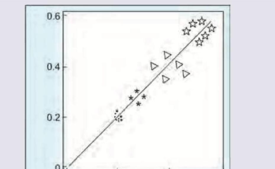
A new diagnostic test is introduced. Based on the image provided showing performance curves of both tests, what characteristics does the new test demonstrate compared to the old one?
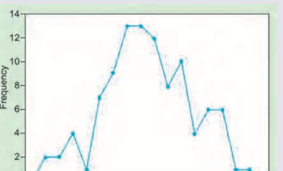
Which type of statistical graph is shown in the image below?
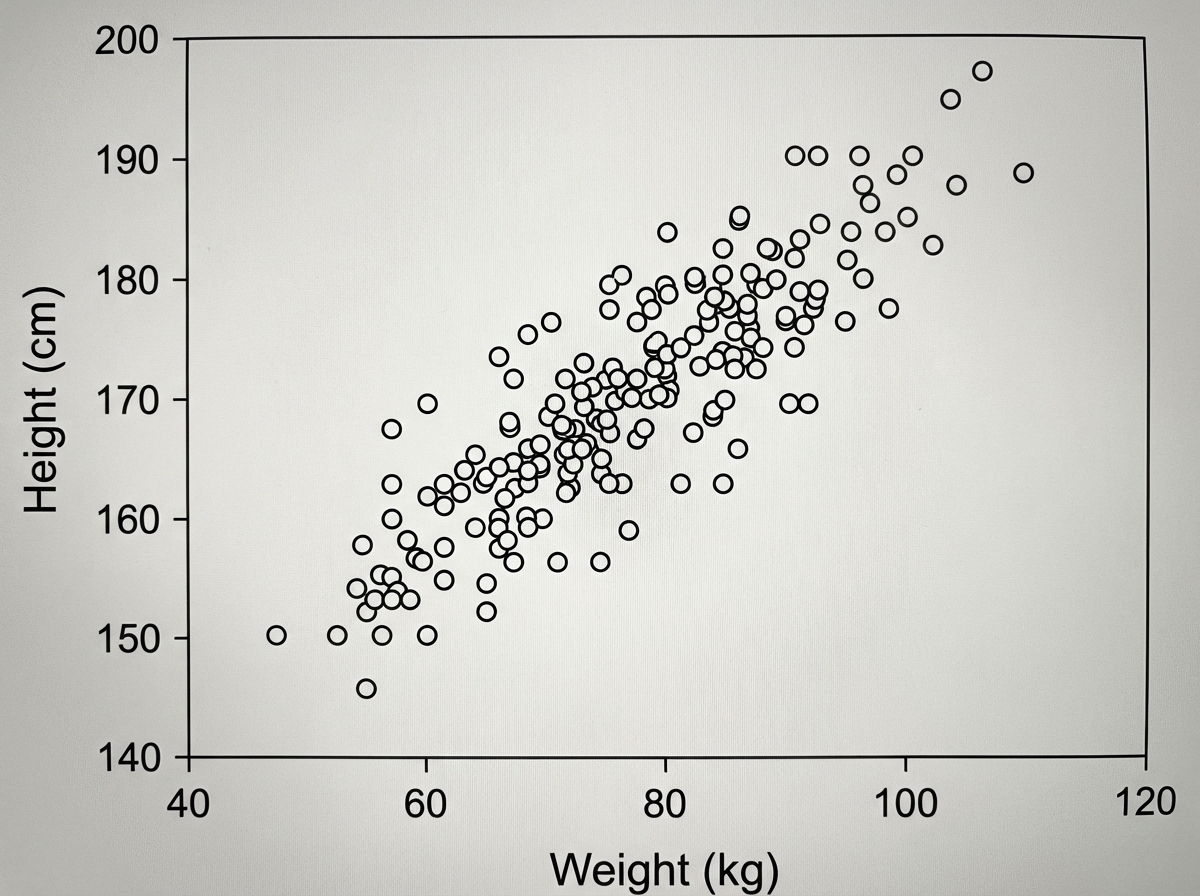
The following scatter plot of 4 different samples shows the correlation between weight and height in the samples. All 4 samples have the same coefficient of correlation of 0.6 taken together, what will be the net correlation coefficient?
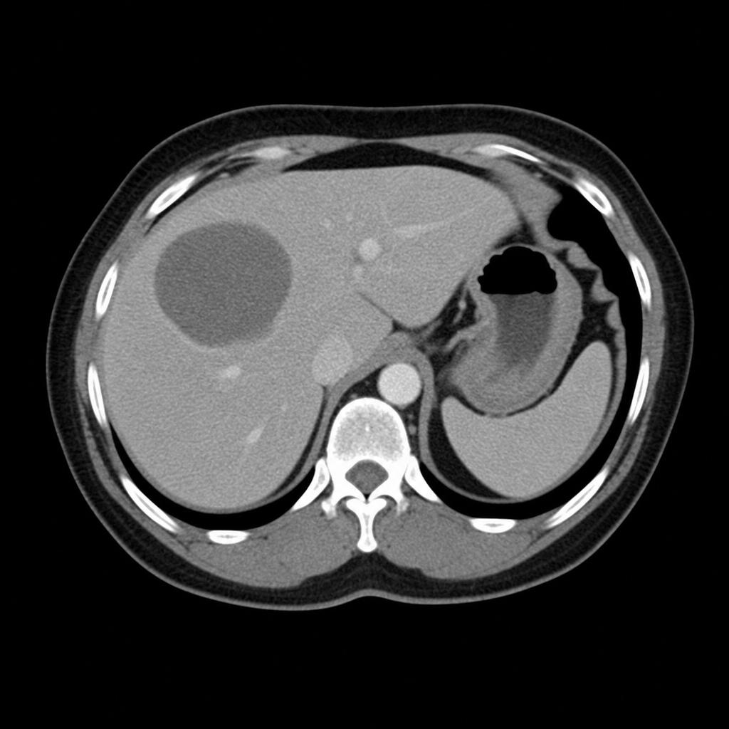
What does the given image show?
What does the following diagram show?
Practice by Chapter
Collection and Presentation of Data
Practice Questions
Measures of Central Tendency
Practice Questions
Measures of Dispersion
Practice Questions
Normal Distribution
Practice Questions
Sampling Methods
Practice Questions
Sample Size Calculation
Practice Questions
Hypothesis Testing
Practice Questions
Tests of Significance
Practice Questions
Correlation and Regression
Practice Questions
Survival Analysis
Practice Questions
Multivariate Analysis
Practice Questions
Statistical Software in Research
Practice Questions
Want unlimited practice?
Get full access to all questions, explanations, and performance tracking.
Scan to download app