Study Design — MCQs

Q: A statistician wants to study the effects of a medicine in three groups-humans, animals, and plants. He then selects randomly from these three groups. Which type of sampling is being performed?

Stratified random sampling. ***Stratified random sampling*** - This method involves dividing the population into **distinct subgroups (strata)** based on shared characteristics (in this case, humans, animals, and plants), and then performing a simple random sample within each stratum. - This ensures that all subgroups are proportionally represented in the sample, which is appropriate when studying effects across different biological categories. *Simple random sampling* - This method involves selecting individuals from the entire population **purely by chance**, without first dividing them into subgroups. - It would not guarantee representation from all three distinct groups (humans, animals, and plants), which is essential for studying differential effects. *Systematic sampling* - This involves selecting samples at **regular intervals** from an ordered list or sequence. - This method is not suitable here because the population is divided into distinct, non-ordered groups rather than a continuous sequence. *Cluster sampling* - This method involves dividing the population into **clusters**, then randomly selecting some clusters and sampling all individuals within those selected clusters. - In this scenario, the initial groups (humans, animals, plants) are strata, not clusters, as the intent is to sample from within each group, not to treat the groups themselves as primary sampling units. *Convenience sampling* - This is a **non-probability sampling method** where subjects are selected based on ease of access rather than random selection. - The question explicitly states that random selection is performed from each group, ruling out convenience sampling.

Q: A study was undertaken to establish the relationship between the consumption of a vegetarian or non-vegetarian diet and the presence of diseases. Which statistical test should be used?

Chi-square test. ***Chi-square test*** - The **chi-square test** is appropriate when analyzing the relationship between two **categorical variables**. In this scenario, "diet type" (vegetarian/non-vegetarian) and "presence of disease" (yes/no) are both categorical variables. - This test determines if there is a statistically significant association between the frequency counts of these two variables in a contingency table. *T-test* - A **t-test** is used to compare the **means** of two groups, typically when the dependent variable is continuous. - This test is unsuitable here because the presence of disease and diet type are categorical, not continuous, variables. *ANOVA* - **ANOVA** (Analysis of Variance) is used to compare the **means** of three or more groups, often with a continuous dependent variable. - Similar to the t-test, ANOVA is not applicable as the study involves categorical variables, not the comparison of means across multiple groups. *Fisher's exact test* - **Fisher's exact test** is similar to the chi-square test but specifically used for **small sample sizes** where the expected frequencies in any cell of the contingency table are less than 5. - While it analyzes categorical data, the chi-square test is the more general and commonly preferred test for larger sample sizes, which is generally assumed unless otherwise specified. *Mann-Whitney U test* - The **Mann-Whitney U test** is a non-parametric test used to compare differences between two independent groups when the dependent variable is **ordinal or continuous** but not normally distributed. - This test is not appropriate for analyzing the association between two categorical variables, as it requires at least one variable to have ranked or continuous data.

Q: A group of 80 people is being studied to determine the effect of diet modification on cholesterol levels. To compare the mean cholesterol levels before and after the diet modification in this group, which statistical test should be used?

Paired t-test. ***Paired t-test*** - A **paired t-test** is appropriate for comparing means from two related samples, such as "before" and "after" measurements on the **same individuals**. - It assesses whether there is a statistically significant difference between these **dependent observations**. *Independent t-test* - The independent t-test compares means between **two separate groups** (unrelated samples). - It is inappropriate here because we have **paired data** from the same individuals measured twice, not two independent groups. *McNemar test* - The McNemar test is used for comparing **paired nominal data**, typically in a 2×2 table, for example, before-after changes in a proportion or categorical outcome. - It is not suitable for **continuous data** like cholesterol levels. *Chi-square test* - The chi-square test is used to assess the association between **two categorical variables** or to compare observed frequencies with expected frequencies. - It is not designed for comparing means of **continuous variables** in paired samples. *Wilcoxon signed-rank test* - The Wilcoxon signed-rank test is a **non-parametric alternative to the paired t-test**, used when the data are not normally distributed or when the sample size is small. - While it's used for paired data, the paired t-test is generally preferred when parametric assumptions (like **normality**) can be met, especially with a sample size of 80.

Q: A study recorded the survival times (in months) of 8 patients diagnosed with pancreatic cancer who received a new chemotherapy regimen. The survival times were: 2, 3, 4, 4, 5, 6, 7, 8 months. What is the median survival time for these patients?

4.5. ***4.5*** - The given survival times are already ordered: 2, 3, 4, 4, 5, 6, 7, 8. - Since there is an **even number of observations (n=8)**, the median is the average of the two middle values, which are the 4th and 5th values. (4 + 5) / 2 = **4.5**. *3.5* - This value would result from incorrectly averaging the 3rd and 4th observations (3 + 4) / 2 = 3.5. - This error occurs when miscounting the middle positions in an even-numbered dataset. *4.0* - This value represents the **fourth observation** in the ordered list, not the true median for an even number of data points. - While it is one of the middle values, the median for an even dataset requires averaging the two middle-most values. *5.0* - This value represents the **fifth observation** in the ordered list, not the true median for an even number of data points. - It would be the median if the dataset contained an odd number of observations and 5 was the middle term. *5.5* - This value would be the mean of 5 and 6, which are the 5th and 6th values, not the correct middle values. - This calculation does not represent the correct methodology for finding the median in this dataset.

Q: An investigator has conducted a prospective study to evaluate the relationship between asthma and the risk of myocardial infarction (MI). She stratifies her analyses by biological sex and observed that among female patients, asthma was a significant predictor of MI risk (hazard ratio = 1.32, p < 0.001). However, among male patients, no relationship was found between asthma and MI risk (p = 0.23). Which of the following best explains the difference observed between male and female patients?

Effect modification. ***Effect modification*** - **Effect modification** occurs when the relationship between an exposure (asthma) and an outcome (MI) differs across various levels of a third variable (biological sex). - In this scenario, sex alters the effect of asthma on MI risk, showing a significant relationship in females but not in males, which is the definition of effect modification. *Measurement bias* - **Measurement bias** refers to systematic errors in the collection of data, leading to inaccurate assessment of exposure, outcome, or confounders. - There is no indication in the question that the methods of measuring asthma or MI differed systematically between males and females, or that the measurements themselves were flawed. *Stratified sampling* - **Stratified sampling** is a technique used in study design where a population is divided into subgroups (strata) and then samples are randomly selected from each stratum. - While the analysis was stratified by sex, this choice was made during data analysis to understand differences, not necessarily during the initial sampling process to ensure representation. *Confounding* - **Confounding** occurs when a third variable is associated with both the exposure and the outcome, and it distorts the true relationship between them. - The investigator stratified by sex and found different results, implying that sex is not merely a confounder that needs to be controlled, but rather a variable that modifies the effect. *Random error* - **Random error** is unsystematic variation in data that can lead to imprecise measurements or findings due to chance. - While random error can contribute to non-significant findings, the significant p-value (<0.001) in females and the clear difference in effect between sexes suggest a systematic phenomenon rather than mere random chance.

Q: A doctor is interested in developing a new over-the-counter medication that can decrease the symptomatic interval of upper respiratory infections from viral etiologies. The doctor wants one group of affected patients to receive the new treatment, but he wants another group of affected patients to not be given the treatment. Of the following clinical trial subtypes, which would be most appropriate in comparing the differences in outcome between the two groups?

Randomized controlled trial. ***Randomized controlled trial*** - This design is ideal for evaluating the **efficacy of an intervention** (new medication) by randomly assigning participants to either a treatment group or a control group. - **Randomization minimizes bias** and ensures that any observed differences in outcomes between the groups can be attributed to the intervention. *Case-control study* - This study design is retrospective and compares individuals with a **disease (cases)** to individuals without the disease (controls) to identify **risk factors** or exposures. - It would not be suitable for testing the effectiveness of a new treatment as it starts with outcomes and looks backward at exposures, not forward at intervention effects. *Cohort study* - A cohort study observes a group of individuals (a cohort) over time to see who develops a disease or outcome, often starting with individuals exposed and unexposed to a **risk factor**. - While it tracks outcomes, it usually doesn't involve an active intervention or random assignment, making it less suitable for directly comparing a new treatment's efficacy against a control. *Historical cohort study* - This is a type of cohort study that uses **past data or records** to identify the cohort and their exposures, then follows them forward in time using existing data to determine outcomes. - It would not be appropriate for testing a *new* medication because it relies on historical exposures and outcomes, not a prospective, controlled intervention. *Cross-sectional study* - This study measures the **prevalence of a disease or condition** and related factors at a single point in time, essentially taking a "snapshot." - It cannot establish causality or evaluate the effectiveness of an intervention over time due to its lack of follow-up and inability to determine the temporal sequence of events.

Q: A 23-year-old woman presents to her primary care physician because she has been having difficulty seeing despite previously having perfect vision all her life. Specifically, she notes that reading, driving, and recognizing faces has become difficult, and she feels that her vision has become fuzzy. She is worried because both of her older brothers have had visual loss with a similar presentation. Visual exam reveals bilateral loss of central vision with decreased visual acuity and color perception. Pathological examination of this patient's retinas reveals degeneration of retinal ganglion cells bilaterally. She is then referred to a geneticist because she wants to know the probability that her son and daughter will also be affected by this disorder. Her husband's family has no history of this disease. Ignoring the effects of incomplete penetrance, which of the following are the chances that this patient's children will be affected by this disease?

Daughter: 100% and son 100%. ***Daughter: 100% and son: 100%*** - This scenario describes **Leber Hereditary Optic Neuropathy (LHON)**, characterized by **bilateral central vision loss** and **degeneration of retinal ganglion cells**, with a maternal inheritance pattern. - LHON is caused by a **mitochondrial DNA mutation**, meaning the disease is transmitted exclusively from the mother to **all her children, regardless of sex**. - Since mitochondrial DNA is inherited entirely from the maternal lineage, **100% of offspring will inherit the mutation**. - The question specifies "ignoring incomplete penetrance," meaning we focus on mutation inheritance rather than symptom development. *Daughter: 50% and son: 50%* - This inheritance pattern is characteristic of an **autosomal dominant** trait, where there is a 50% chance of passing the allele to each child. - This does not fit the described pattern of maternal inheritance where all children inherit the mutation from an affected mother. *Daughter: ~0% and son: ~0%* - This would only be true if neither parent was a carrier or affected, or if the disease had a very complex, non-mendelian inheritance with low penetrance. - Given the mother's affected status and the mitochondrial inheritance pattern, the children will definitely inherit the mutation. *Daughter: 25% and son: 25%* - This ratio is typical for an **autosomal recessive** inheritance pattern where both parents are heterozygotes (carriers). - This does not align with the exclusively maternal transmission observed in LHON. *Daughter: ~0% and son: 50%* - This inheritance pattern is typical for an **X-linked recessive** disorder, where daughters of an affected father are unaffected carriers and sons have a 50% chance of being affected if the mother is a carrier. - This is incorrect because LHON is mitochondrially inherited from the mother to all children, not X-linked.

Q: A group of researchers recently conducted a meta-analysis of twenty clinical trials encompassing 10,000 women with estrogen receptor-positive breast cancer who were disease-free following adjuvant radiotherapy. After an observation period of 15 years, the relationship between tumor grade and distant recurrence of cancer was evaluated. The results show: Distant recurrence No distant recurrence Well differentiated 500 4500 Moderately differentiated 375 2125 Poorly differentiated 550 1950 Based on this information, which of the following is the 15-year risk for distant recurrence in patients with high-grade breast cancer?

550/2500. ***550/2500*** - The question asks for the 15-year risk for distant recurrence in patients with **high-grade breast cancer**, which corresponds to **poorly differentiated** tumors in the provided data. - For poorly differentiated tumors, there were 550 cases of distant recurrence out of a total of 550 + 1950 = **2500 patients** (550 with recurrence + 1950 without recurrence). Therefore, the risk is 550/2500. *500/5000* - This calculation represents the risk for distant recurrence in **well-differentiated** tumors (500 recurrences out of 500 + 4500 = 5000 total well-differentiated cases), not high-grade (poorly differentiated) tumors. *1950/8575* - This calculation incorrectly uses 1950 (number of poorly differentiated patients *without* recurrence) as the numerator. The denominator also appears to be incorrectly calculated or irrelevant to the specific group in question. *2500/10000* - This calculation represents the **total number of poorly differentiated patients** (2500) divided by the total number of patients in the study (10000), which is the proportion of patients with poorly differentiated cancer, not the risk of recurrence within that group. *550/1425* - This calculation incorrectly uses 1425 as the denominator. The total number of patients with poorly differentiated tumors is 2500 (550 with recurrence + 1950 without recurrence), not 1425.

Q: A clinical trial is conducted to determine the role of cerebrospinal fluid (CSF) beta-amyloid levels as a biomarker in the early detection and prognosis of Alzheimer disease. A total of 100 participants are enrolled and separated into three groups according to their Mini-Mental State Examination (MMSE) score: mild dementia (20–24 points), moderate dementia (13–20 points), and severe dementia (< 13 points). Participants' CSF level of beta-amyloid 42 is measured using an immunoassay. It is found that participants with severe dementia have a statistically significantly lower mean CSF level of beta-amyloid 42 compared to the other two groups. Which of the following statistical tests was most likely used to compare measurements between the study groups?

Analysis of variance. ***Analysis of variance (ANOVA)*** - This statistical test is used to compare the means of **three or more independent groups**. In this scenario, it would be appropriate for comparing the mean CSF beta-amyloid levels across the mild, moderate, and severe dementia groups. - ANOVA determines if there is a statistically significant difference between the means of these groups, and if so, post-hoc tests can identify which specific groups differ. *Chi-square test* - The chi-square test is used for **categorical data** to determine if there is a significant association between two variables. - This scenario involves comparing **continuous numerical data** (CSF beta-amyloid levels) across groups, not categorical frequencies. *Pearson correlation analysis* - Pearson correlation measures the **linear relationship** and strength of association between **two continuous numerical variables**. - Here, the goal is to compare means across multiple groups, not to assess the correlation between two continuous variables. *Fisher's exact test* - Fisher's exact test is used for analyzing the association between two **categorical variables** in a **2x2 contingency table**, especially with small sample sizes. - This test is not suitable for comparing the means of a continuous variable across multiple groups. *Two-sample t-test* - A two-sample t-test is used to compare the means of **exactly two independent groups**. - Since this study involves **three distinct groups** (mild, moderate, and severe dementia), a two-sample t-test would be insufficient to analyze all group comparisons simultaneously, requiring multiple t-tests which increases the risk of Type I error.

An investigator has conducted a prospective study to evaluate the relationship between asthma and the risk of myocardial infarction (MI). She stratifies her analyses by biological sex and observed that among female patients, asthma was a significant predictor of MI risk (hazard ratio = 1.32, p < 0.001). However, among male patients, no relationship was found between asthma and MI risk (p = 0.23). Which of the following best explains the difference observed between male and female patients?

An investigator studying the effects of dietary salt restriction on atrial fibrillation compares two published studies, A and B. In study A, nursing home patients without atrial fibrillation were randomly assigned to a treatment group receiving a low-salt diet or a control group without dietary salt restriction. When study B began, dietary sodium intake was estimated among elderly outpatients without atrial fibrillation using 24-hour dietary recall. In both studies, patients were reevaluated at the end of one year for atrial fibrillation. Which of the following statements about the two studies is true?

A doctor is interested in developing a new over-the-counter medication that can decrease the symptomatic interval of upper respiratory infections from viral etiologies. The doctor wants one group of affected patients to receive the new treatment, but he wants another group of affected patients to not be given the treatment. Of the following clinical trial subtypes, which would be most appropriate in comparing the differences in outcome between the two groups?

A 23-year-old woman presents to her primary care physician because she has been having difficulty seeing despite previously having perfect vision all her life. Specifically, she notes that reading, driving, and recognizing faces has become difficult, and she feels that her vision has become fuzzy. She is worried because both of her older brothers have had visual loss with a similar presentation. Visual exam reveals bilateral loss of central vision with decreased visual acuity and color perception. Pathological examination of this patient's retinas reveals degeneration of retinal ganglion cells bilaterally. She is then referred to a geneticist because she wants to know the probability that her son and daughter will also be affected by this disorder. Her husband's family has no history of this disease. Ignoring the effects of incomplete penetrance, which of the following are the chances that this patient's children will be affected by this disease?

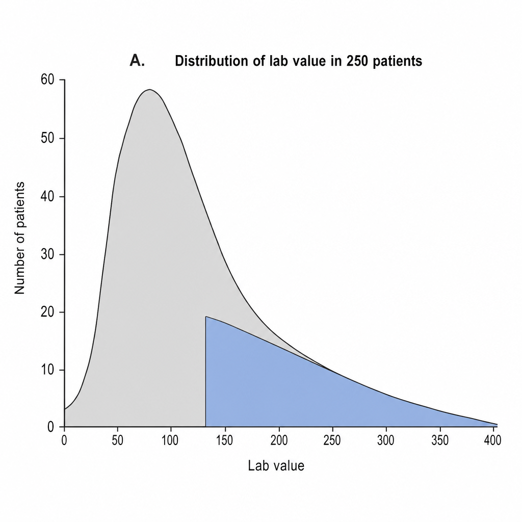
A group of researchers recently conducted a meta-analysis of twenty clinical trials encompassing 10,000 women with estrogen receptor-positive breast cancer who were disease-free following adjuvant radiotherapy. After an observation period of 15 years, the relationship between tumor grade and distant recurrence of cancer was evaluated. The results show: Distant recurrence No distant recurrence Well differentiated 500 4500 Moderately differentiated 375 2125 Poorly differentiated 550 1950 Based on this information, which of the following is the 15-year risk for distant recurrence in patients with high-grade breast cancer?

Q10

A clinical trial is conducted to determine the role of cerebrospinal fluid (CSF) beta-amyloid levels as a biomarker in the early detection and prognosis of Alzheimer disease. A total of 100 participants are enrolled and separated into three groups according to their Mini-Mental State Examination (MMSE) score: mild dementia (20–24 points), moderate dementia (13–20 points), and severe dementia (< 13 points). Participants' CSF level of beta-amyloid 42 is measured using an immunoassay. It is found that participants with severe dementia have a statistically significantly lower mean CSF level of beta-amyloid 42 compared to the other two groups. Which of the following statistical tests was most likely used to compare measurements between the study groups?

Study Design US Medical PG Practice Questions and MCQs

Question 1: A statistician wants to study the effects of a medicine in three groups-humans, animals, and plants. He then selects randomly from these three groups. Which type of sampling is being performed?

A. Simple random sampling
B. Systematic sampling
C. Stratified random sampling (Correct Answer)
D. Cluster sampling
E. Convenience sampling

Explanation: ***Stratified random sampling*** - This method involves dividing the population into **distinct subgroups (strata)** based on shared characteristics (in this case, humans, animals, and plants), and then performing a simple random sample within each stratum. - This ensures that all subgroups are proportionally represented in the sample, which is appropriate when studying effects across different biological categories. *Simple random sampling* - This method involves selecting individuals from the entire population **purely by chance**, without first dividing them into subgroups. - It would not guarantee representation from all three distinct groups (humans, animals, and plants), which is essential for studying differential effects. *Systematic sampling* - This involves selecting samples at **regular intervals** from an ordered list or sequence. - This method is not suitable here because the population is divided into distinct, non-ordered groups rather than a continuous sequence. *Cluster sampling* - This method involves dividing the population into **clusters**, then randomly selecting some clusters and sampling all individuals within those selected clusters. - In this scenario, the initial groups (humans, animals, plants) are strata, not clusters, as the intent is to sample from within each group, not to treat the groups themselves as primary sampling units. *Convenience sampling* - This is a **non-probability sampling method** where subjects are selected based on ease of access rather than random selection. - The question explicitly states that random selection is performed from each group, ruling out convenience sampling.

Question 2: A study was undertaken to establish the relationship between the consumption of a vegetarian or non-vegetarian diet and the presence of diseases. Which statistical test should be used?

A. Chi-square test (Correct Answer)
B. T-test
C. ANOVA
D. Fisher's exact test
E. Mann-Whitney U test

Explanation: ***Chi-square test*** - The **chi-square test** is appropriate when analyzing the relationship between two **categorical variables**. In this scenario, "diet type" (vegetarian/non-vegetarian) and "presence of disease" (yes/no) are both categorical variables. - This test determines if there is a statistically significant association between the frequency counts of these two variables in a contingency table. *T-test* - A **t-test** is used to compare the **means** of two groups, typically when the dependent variable is continuous. - This test is unsuitable here because the presence of disease and diet type are categorical, not continuous, variables. *ANOVA* - **ANOVA** (Analysis of Variance) is used to compare the **means** of three or more groups, often with a continuous dependent variable. - Similar to the t-test, ANOVA is not applicable as the study involves categorical variables, not the comparison of means across multiple groups. *Fisher's exact test* - **Fisher's exact test** is similar to the chi-square test but specifically used for **small sample sizes** where the expected frequencies in any cell of the contingency table are less than 5. - While it analyzes categorical data, the chi-square test is the more general and commonly preferred test for larger sample sizes, which is generally assumed unless otherwise specified. *Mann-Whitney U test* - The **Mann-Whitney U test** is a non-parametric test used to compare differences between two independent groups when the dependent variable is **ordinal or continuous** but not normally distributed. - This test is not appropriate for analyzing the association between two categorical variables, as it requires at least one variable to have ranked or continuous data.

Question 3: A group of 80 people is being studied to determine the effect of diet modification on cholesterol levels. To compare the mean cholesterol levels before and after the diet modification in this group, which statistical test should be used?

A. Paired t-test (Correct Answer)
B. McNemar test
C. Chi-square test
D. Wilcoxon signed-rank test
E. Independent t-test

Explanation: ***Paired t-test*** - A **paired t-test** is appropriate for comparing means from two related samples, such as "before" and "after" measurements on the **same individuals**. - It assesses whether there is a statistically significant difference between these **dependent observations**. *Independent t-test* - The independent t-test compares means between **two separate groups** (unrelated samples). - It is inappropriate here because we have **paired data** from the same individuals measured twice, not two independent groups. *McNemar test* - The McNemar test is used for comparing **paired nominal data**, typically in a 2×2 table, for example, before-after changes in a proportion or categorical outcome. - It is not suitable for **continuous data** like cholesterol levels. *Chi-square test* - The chi-square test is used to assess the association between **two categorical variables** or to compare observed frequencies with expected frequencies. - It is not designed for comparing means of **continuous variables** in paired samples. *Wilcoxon signed-rank test* - The Wilcoxon signed-rank test is a **non-parametric alternative to the paired t-test**, used when the data are not normally distributed or when the sample size is small. - While it's used for paired data, the paired t-test is generally preferred when parametric assumptions (like **normality**) can be met, especially with a sample size of 80.

Question 4: A study recorded the survival times (in months) of 8 patients diagnosed with pancreatic cancer who received a new chemotherapy regimen. The survival times were: 2, 3, 4, 4, 5, 6, 7, 8 months. What is the median survival time for these patients?

A. 4.0
B. 4.5 (Correct Answer)
C. 5.0
D. 5.5
E. 3.5

Explanation: ***4.5*** - The given survival times are already ordered: 2, 3, 4, 4, 5, 6, 7, 8. - Since there is an **even number of observations (n=8)**, the median is the average of the two middle values, which are the 4th and 5th values. (4 + 5) / 2 = **4.5**. *3.5* - This value would result from incorrectly averaging the 3rd and 4th observations (3 + 4) / 2 = 3.5. - This error occurs when miscounting the middle positions in an even-numbered dataset. *4.0* - This value represents the **fourth observation** in the ordered list, not the true median for an even number of data points. - While it is one of the middle values, the median for an even dataset requires averaging the two middle-most values. *5.0* - This value represents the **fifth observation** in the ordered list, not the true median for an even number of data points. - It would be the median if the dataset contained an odd number of observations and 5 was the middle term. *5.5* - This value would be the mean of 5 and 6, which are the 5th and 6th values, not the correct middle values. - This calculation does not represent the correct methodology for finding the median in this dataset.

Question 5: An investigator has conducted a prospective study to evaluate the relationship between asthma and the risk of myocardial infarction (MI). She stratifies her analyses by biological sex and observed that among female patients, asthma was a significant predictor of MI risk (hazard ratio = 1.32, p < 0.001). However, among male patients, no relationship was found between asthma and MI risk (p = 0.23). Which of the following best explains the difference observed between male and female patients?

A. Effect modification (Correct Answer)
B. Measurement bias
C. Stratified sampling
D. Confounding
E. Random error

Explanation: ***Effect modification*** - **Effect modification** occurs when the relationship between an exposure (asthma) and an outcome (MI) differs across various levels of a third variable (biological sex). - In this scenario, sex alters the effect of asthma on MI risk, showing a significant relationship in females but not in males, which is the definition of effect modification. *Measurement bias* - **Measurement bias** refers to systematic errors in the collection of data, leading to inaccurate assessment of exposure, outcome, or confounders. - There is no indication in the question that the methods of measuring asthma or MI differed systematically between males and females, or that the measurements themselves were flawed. *Stratified sampling* - **Stratified sampling** is a technique used in study design where a population is divided into subgroups (strata) and then samples are randomly selected from each stratum. - While the analysis was stratified by sex, this choice was made during data analysis to understand differences, not necessarily during the initial sampling process to ensure representation. *Confounding* - **Confounding** occurs when a third variable is associated with both the exposure and the outcome, and it distorts the true relationship between them. - The investigator stratified by sex and found different results, implying that sex is not merely a confounder that needs to be controlled, but rather a variable that modifies the effect. *Random error* - **Random error** is unsystematic variation in data that can lead to imprecise measurements or findings due to chance. - While random error can contribute to non-significant findings, the significant p-value (<0.001) in females and the clear difference in effect between sexes suggest a systematic phenomenon rather than mere random chance.

Question 6: An investigator studying the effects of dietary salt restriction on atrial fibrillation compares two published studies, A and B. In study A, nursing home patients without atrial fibrillation were randomly assigned to a treatment group receiving a low-salt diet or a control group without dietary salt restriction. When study B began, dietary sodium intake was estimated among elderly outpatients without atrial fibrillation using 24-hour dietary recall. In both studies, patients were reevaluated at the end of one year for atrial fibrillation. Which of the following statements about the two studies is true?

A. Study A results can be analyzed using a t-test
B. Study B results can be analyzed using a chi-square test
C. Study A allows for better control of confounding variables (Correct Answer)
D. Study B allows for better control over selection bias
E. Study B is better at inferring causality

Explanation: ***Study A allows for better control of confounding variables*** - **Random assignment** in Study A helps distribute both known and unknown confounding variables equally between the treatment and control groups, thereby minimizing their impact on the observed outcome. - Unlike Study B, which is observational, Study A's experimental design creates comparable groups, allowing for a more accurate assessment of the direct effect of the intervention. *Study A results can be analyzed using a t-test* - A **t-test** is typically used to compare the means of two groups for a **continuous outcome variable**. - The outcome variable in this study, the presence or absence of **atrial fibrillation**, is a **dichotomous (categorical) variable**, making a t-test inappropriate. - The correct statistical test would be a **chi-square test** or **Fisher's exact test**. *Study B results can be analyzed using a chi-square test* - While technically a **chi-square test** could be used to analyze the association between categorized dietary sodium intake and atrial fibrillation in Study B, this statement is not the **best answer** to the question. - The question asks which statement is **most characteristically true** when comparing the two studies, and Study A's superior control of confounding variables through randomization is the most defining difference between an RCT and an observational cohort study. - Additionally, cohort studies typically report **relative risk** or **hazard ratios** rather than simple chi-square associations. *Study B allows for better control over selection bias* - Study B is an **observational cohort study** that relies on existing groups of outpatients, making it susceptible to **selection bias** as participants are not randomly assigned. - The method of recruiting outpatients without randomization can introduce differences between groups that are not accounted for, leading to biased results. *Study B is better at inferring causality* - Study B, being an **observational cohort study**, can only identify **associations** between dietary salt intake and atrial fibrillation, not establish a **causal relationship**. - The lack of **randomization** means that other unmeasured factors might be responsible for any observed association, making causal inference unreliable.

Question 7: A doctor is interested in developing a new over-the-counter medication that can decrease the symptomatic interval of upper respiratory infections from viral etiologies. The doctor wants one group of affected patients to receive the new treatment, but he wants another group of affected patients to not be given the treatment. Of the following clinical trial subtypes, which would be most appropriate in comparing the differences in outcome between the two groups?

A. Randomized controlled trial (Correct Answer)
B. Case-control study
C. Cohort study
D. Historical cohort study
E. Cross-sectional study

Explanation: ***Randomized controlled trial*** - This design is ideal for evaluating the **efficacy of an intervention** (new medication) by randomly assigning participants to either a treatment group or a control group. - **Randomization minimizes bias** and ensures that any observed differences in outcomes between the groups can be attributed to the intervention. *Case-control study* - This study design is retrospective and compares individuals with a **disease (cases)** to individuals without the disease (controls) to identify **risk factors** or exposures. - It would not be suitable for testing the effectiveness of a new treatment as it starts with outcomes and looks backward at exposures, not forward at intervention effects. *Cohort study* - A cohort study observes a group of individuals (a cohort) over time to see who develops a disease or outcome, often starting with individuals exposed and unexposed to a **risk factor**. - While it tracks outcomes, it usually doesn't involve an active intervention or random assignment, making it less suitable for directly comparing a new treatment's efficacy against a control. *Historical cohort study* - This is a type of cohort study that uses **past data or records** to identify the cohort and their exposures, then follows them forward in time using existing data to determine outcomes. - It would not be appropriate for testing a *new* medication because it relies on historical exposures and outcomes, not a prospective, controlled intervention. *Cross-sectional study* - This study measures the **prevalence of a disease or condition** and related factors at a single point in time, essentially taking a "snapshot." - It cannot establish causality or evaluate the effectiveness of an intervention over time due to its lack of follow-up and inability to determine the temporal sequence of events.

Question 8: A 23-year-old woman presents to her primary care physician because she has been having difficulty seeing despite previously having perfect vision all her life. Specifically, she notes that reading, driving, and recognizing faces has become difficult, and she feels that her vision has become fuzzy. She is worried because both of her older brothers have had visual loss with a similar presentation. Visual exam reveals bilateral loss of central vision with decreased visual acuity and color perception. Pathological examination of this patient's retinas reveals degeneration of retinal ganglion cells bilaterally. She is then referred to a geneticist because she wants to know the probability that her son and daughter will also be affected by this disorder. Her husband's family has no history of this disease. Ignoring the effects of incomplete penetrance, which of the following are the chances that this patient's children will be affected by this disease?

A. Daughter: 50% and son: 50%
B. Daughter: ~0% and son: ~0%
C. Daughter: 25% and son: 25%
D. Daughter: ~0% and son: 50%
E. Daughter: 100% and son 100% (Correct Answer)

Explanation: ***Daughter: 100% and son: 100%*** - This scenario describes **Leber Hereditary Optic Neuropathy (LHON)**, characterized by **bilateral central vision loss** and **degeneration of retinal ganglion cells**, with a maternal inheritance pattern. - LHON is caused by a **mitochondrial DNA mutation**, meaning the disease is transmitted exclusively from the mother to **all her children, regardless of sex**. - Since mitochondrial DNA is inherited entirely from the maternal lineage, **100% of offspring will inherit the mutation**. - The question specifies "ignoring incomplete penetrance," meaning we focus on mutation inheritance rather than symptom development. *Daughter: 50% and son: 50%* - This inheritance pattern is characteristic of an **autosomal dominant** trait, where there is a 50% chance of passing the allele to each child. - This does not fit the described pattern of maternal inheritance where all children inherit the mutation from an affected mother. *Daughter: ~0% and son: ~0%* - This would only be true if neither parent was a carrier or affected, or if the disease had a very complex, non-mendelian inheritance with low penetrance. - Given the mother's affected status and the mitochondrial inheritance pattern, the children will definitely inherit the mutation. *Daughter: 25% and son: 25%* - This ratio is typical for an **autosomal recessive** inheritance pattern where both parents are heterozygotes (carriers). - This does not align with the exclusively maternal transmission observed in LHON. *Daughter: ~0% and son: 50%* - This inheritance pattern is typical for an **X-linked recessive** disorder, where daughters of an affected father are unaffected carriers and sons have a 50% chance of being affected if the mother is a carrier. - This is incorrect because LHON is mitochondrially inherited from the mother to all children, not X-linked.

Question 9: A group of researchers recently conducted a meta-analysis of twenty clinical trials encompassing 10,000 women with estrogen receptor-positive breast cancer who were disease-free following adjuvant radiotherapy. After an observation period of 15 years, the relationship between tumor grade and distant recurrence of cancer was evaluated. The results show: Distant recurrence No distant recurrence Well differentiated 500 4500 Moderately differentiated 375 2125 Poorly differentiated 550 1950 Based on this information, which of the following is the 15-year risk for distant recurrence in patients with high-grade breast cancer?

A. 500/5000
B. 1950/8575
C. 550/2500 (Correct Answer)
D. 2500/10000
E. 550/1425

Explanation: ***550/2500*** - The question asks for the 15-year risk for distant recurrence in patients with **high-grade breast cancer**, which corresponds to **poorly differentiated** tumors in the provided data. - For poorly differentiated tumors, there were 550 cases of distant recurrence out of a total of 550 + 1950 = **2500 patients** (550 with recurrence + 1950 without recurrence). Therefore, the risk is 550/2500. *500/5000* - This calculation represents the risk for distant recurrence in **well-differentiated** tumors (500 recurrences out of 500 + 4500 = 5000 total well-differentiated cases), not high-grade (poorly differentiated) tumors. *1950/8575* - This calculation incorrectly uses 1950 (number of poorly differentiated patients *without* recurrence) as the numerator. The denominator also appears to be incorrectly calculated or irrelevant to the specific group in question. *2500/10000* - This calculation represents the **total number of poorly differentiated patients** (2500) divided by the total number of patients in the study (10000), which is the proportion of patients with poorly differentiated cancer, not the risk of recurrence within that group. *550/1425* - This calculation incorrectly uses 1425 as the denominator. The total number of patients with poorly differentiated tumors is 2500 (550 with recurrence + 1950 without recurrence), not 1425.

Question 10: A clinical trial is conducted to determine the role of cerebrospinal fluid (CSF) beta-amyloid levels as a biomarker in the early detection and prognosis of Alzheimer disease. A total of 100 participants are enrolled and separated into three groups according to their Mini-Mental State Examination (MMSE) score: mild dementia (20–24 points), moderate dementia (13–20 points), and severe dementia (< 13 points). Participants' CSF level of beta-amyloid 42 is measured using an immunoassay. It is found that participants with severe dementia have a statistically significantly lower mean CSF level of beta-amyloid 42 compared to the other two groups. Which of the following statistical tests was most likely used to compare measurements between the study groups?

A. Chi-square test
B. Pearson correlation analysis
C. Analysis of variance (Correct Answer)
D. Two-sample t-test
E. Fisher's exact test

Explanation: ***Analysis of variance (ANOVA)*** - This statistical test is used to compare the means of **three or more independent groups**. In this scenario, it would be appropriate for comparing the mean CSF beta-amyloid levels across the mild, moderate, and severe dementia groups. - ANOVA determines if there is a statistically significant difference between the means of these groups, and if so, post-hoc tests can identify which specific groups differ. *Chi-square test* - The chi-square test is used for **categorical data** to determine if there is a significant association between two variables. - This scenario involves comparing **continuous numerical data** (CSF beta-amyloid levels) across groups, not categorical frequencies. *Pearson correlation analysis* - Pearson correlation measures the **linear relationship** and strength of association between **two continuous numerical variables**. - Here, the goal is to compare means across multiple groups, not to assess the correlation between two continuous variables. *Fisher's exact test* - Fisher's exact test is used for analyzing the association between two **categorical variables** in a **2x2 contingency table**, especially with small sample sizes. - This test is not suitable for comparing the means of a continuous variable across multiple groups. *Two-sample t-test* - A two-sample t-test is used to compare the means of **exactly two independent groups**. - Since this study involves **three distinct groups** (mild, moderate, and severe dementia), a two-sample t-test would be insufficient to analyze all group comparisons simultaneously, requiring multiple t-tests which increases the risk of Type I error.

Question 11: A 4th grade class in Salem, Massachusetts has 20 students. Due to recent media coverage of the fallacious association between vaccines and autism, none of the students have been immunized against influenza this year. Fortunately, up to this point none of the students has come down with the flu. During the first week of flu season, however, 2 students contract influenza. In the second week, 3 more students contract influenza. And in the third week, 5 more students contract influenza. The other students remained healthy throughout the rest of the flu season. In this class, what was the risk of contracting influenza during the second week of the flu season?

A. 0.1
B. 0.5
C. 0.15
D. 0.25
E. 0.17 (Correct Answer)

Explanation: ***0.17*** - To calculate the risk during the second week, we need the number of new cases in that week (3 students) and the number of **at-risk individuals** at the beginning of that week. - At the start of the second week, 18 students were at risk (20 total - 2 who contracted flu in the first week). Therefore, risk = 3/18 = **0.1666**, which rounds to **0.17**. - This correctly applies the formula: **Risk = (new cases) / (population at risk at start of period)**. *0.1* - This value would imply 2 new cases out of 20 students, or similar miscalculation. - This does not correctly account for the **dynamically changing population at risk** and uses wrong numerator or denominator. *0.15* - This incorrectly uses 20 as the denominator (3/20 = 0.15), failing to exclude the 2 students who already had influenza. - The **population at risk must exclude those already diseased** at the start of the time period. *0.25* - This fraction could represent 5 new cases out of 20 total students, or 3 new cases out of 12 students. - This answer does not reflect the **specific incidence** during the second week with the correct denominator. *0.5* - This would mean half of the population contracted influenza, which is significantly higher than the observed 3 new cases in the second week. - This value is a gross **overestimation of the actual risk** during the specified period.

Question 12: You are interested in tracking the disease burden of a highly contagious viral disease over a time period of 5 years. The virus appears to be indigenous to rural parts of northern Africa. Which of the following research study designs would be optimal for your analysis?

A. Case series
B. Case-control
C. Cohort study (Correct Answer)
D. Cross-sectional
E. Randomized controlled trial

Explanation: ***Cohort study*** - A **cohort study** allows for tracking disease incidence and progression over a defined period (5 years) in a group of individuals (cohort) exposed to conditions in rural Northern Africa, making it optimal for assessing disease burden over time. - This design is ideal for investigating the natural history of a disease and identifying risk factors within a specific population. *Case series* - A **case series** describes characteristics of a group of patients with a particular disease and is useful for hypothesis generation rather than tracking disease burden over time. - It lacks a comparison group, making it unsuitable for assessing incidence or prevalence in a population. *Case-control* - A **case-control study** compares individuals with a disease (cases) to individuals without the disease (controls) and looks retrospectively for exposure differences to identify risk factors. - This design is efficient for rare diseases but less suitable for tracking overall disease burden or incidence trends over a long period. *Cross-sectional* - A **cross-sectional study** measures the prevalence of disease and exposure at a single point in time, providing a snapshot of the population. - While useful for prevalence, it cannot establish temporality or track changes in disease burden over a 5-year period. *Randomized controlled trial* - A **randomized controlled trial (RCT)** is designed to evaluate the effectiveness of an intervention by randomly assigning participants to treatment or control groups. - This design is unethical and impractical for tracking the natural disease burden of an indigenous viral disease in a population.

Question 13: A researcher faces the task of calculating the mean height of male students in an undergraduate class containing a total of 2,000 male students and 1,750 female students. The mean height of a sample of male students is computed as 176 cm (69.3 in), with a standard deviation of 7 cm (2.8 in). The researcher now tries to calculate the confidence interval for the mean height of the male students in the undergraduate class. Which additional data will be needed for this calculation?

A. The mean height of all the male students in the undergraduate class
B. The given data are adequate, and no more data are needed.
C. Total sample size of the study (Correct Answer)
D. Total number of male students in the undergraduate class who did not take part in the study
E. A sampling frame of all of the male students in the undergraduate class

Explanation: ***Total sample size of the study*** - To calculate the **confidence interval**, one needs the **sample mean**, **standard deviation**, and critically, the **sample size (n)**. - The sample size is crucial because it influences the **standard error of the mean** and thus the width of the confidence interval. *The mean height of all the male students in the undergraduate class* - This value represents the **true population mean**, which is precisely what the confidence interval is trying to **estimate**. - If this value were known, there would be no need to calculate a confidence interval for it. *The given data are adequate, and no more data are needed.* - While the **sample mean** and **standard deviation** are provided, the problem statement does not explicitly state the **sample size (n)** of male students from which these statistics were derived. - The number of all male students (2,000) is the **population size**, not the sample size used for the calculation. *Total number of male students in the undergraduate class who did not take part in the study* - This information is not directly used in the calculation of a **confidence interval** for the mean. - It relates to the part of the population that was not sampled, which doesn't impact the formula for the confidence interval itself. *A sampling frame of all of the male students in the undergraduate class* - A **sampling frame** is a list of all individuals in the population from which a sample can be drawn; it's essential for the **sampling process** itself. - However, once the sample mean and standard deviation are obtained, the sampling frame is not directly needed for the *calculation* of the confidence interval.

Question 14: You are conducting a systematic review on the effect of a new sulfonylurea for the treatment of type II diabetes. For your systematic review you would like to include 95% confidence intervals for the mean of blood glucose levels in the treatment groups. What further information is necessary to abstract from each of the original papers in order to calculate a 95% confidence interval for each study?

A. Power, standard deviation, mean
B. Power, mean, sample size
C. Standard deviation, mean, sample size (Correct Answer)
D. Standard deviation, mean, sample size, power
E. Power, standard deviation, sample size

Explanation: ***Standard deviation, mean, sample size*** - To calculate a **95% confidence interval** for the mean, you need the **sample mean**, the **standard deviation** (which quantifies data variability), and the **sample size** (the number of observations). - The formula for a confidence interval for the mean involves these three components and a z-score or t-score corresponding to the desired confidence level. *Power, standard deviation, mean* - **Power** is related to the probability of correctly rejecting a false null hypothesis and is not directly used in the calculation of a confidence interval for a single mean. - While **standard deviation** and **mean** are necessary, **sample size** is also crucial for the calculation, which is missing from this option. *Power, mean, sample size* - **Power** is a concept relevant to study design and hypothesis testing, not for calculating a confidence interval for an observed mean. - While **mean** and **sample size** are correctly identified, the **standard deviation** is a critical missing component needed to quantify the variability around the mean. *Standard deviation, mean, sample size, power* - While **standard deviation**, **mean**, and **sample size** are all needed for calculating the confidence interval, **power** is not required for this specific calculation. - Including **power** as a necessary piece of information is incorrect because it relates to the study's ability to detect an effect, not the precision of an estimated mean. *Power, standard deviation, sample size* - This option incorrectly includes **power**, which is not needed for calculating a confidence interval for the mean. - It also omits the **mean** itself, which is a fundamental component of the confidence interval formula as the central estimate.

Question 15: A study looking to examine the utility of colorectal cancer screening in patients younger than 50 is currently seeking subjects to enroll. A 49-year-old man with a family history of colorectal cancer is very interested in enrolling in the study, due to his own personal concerns about developing cancer. If enrolled in this study, which of the following types of biases will this represent?

A. Recall bias
B. Measurement bias
C. Selection bias (Correct Answer)
D. Length bias
E. Lead-time bias

Explanation: ***Selection bias*** - This scenario exemplifies **selection bias** because the individual actively seeks to participate in the study due to personal concerns and a **family history of colorectal cancer**. This means the study participants may not be representative of the general population younger than 50, potentially skewing the results to show a higher prevalence or different screening utility than would be found in a genuinely random sample. - **Selection bias** occurs when the selection of subjects for a study (or their retention in the study) results in a sample that is not truly representative of the target population. *Recall bias* - **Recall bias** occurs when subjects with a particular condition (e.g., CRC) are more likely to remember exposures or risk factors than healthy controls. - This bias is typically a problem in **retrospective studies** where subjects are asked to recall past events. *Measurement bias* - **Measurement bias** arises from flaws in the way data is collected or measured, leading to systematically inaccurate results. - Examples include using **faulty equipment** or inconsistent methods for assessing outcomes or exposures, leading to misclassification. *Length bias* - **Length bias** in screening refers to the fact that screening tests are more likely to detect cases of disease that are **slower-growing** and have a longer preclinical phase. - This can make screened populations appear to have a better prognosis, as the more aggressive, fast-growing cases are often missed between screening intervals. *Lead-time bias* - **Lead-time bias** refers to the apparent increase in survival time among screened individuals due to the **earlier detection of disease** by screening, rather than an actual prolongation of life. - It occurs when the time from diagnosis to death is artificially lengthened because the disease was found earlier, even if the actual date of death remains unchanged.

Question 16: A new antihypertensive medication is studied in 3,000 Caucasian men with coronary heart disease who are over age 65. The results show benefits in terms of improved morbidity and mortality as well as a decreased rate of acute coronary events with minimal side effects. After hearing about this new medication and supporting study at a recent continuing education course, a family physician elects to prescribe this medication to a 39-year-old Hispanic female who presents with primary hypertension. After a one month trial and appropriate adjustments in the dosing, the patient's blood pressure is not well controlled by this medication. Which of the following statistical concepts could explain this patient's poor response to the medication?

A. Effect modification
B. Observer bias
C. Selection bias
D. Confounding
E. Generalizability (Correct Answer)

Explanation: ***Generalizability*** - The study population was very specific (**Caucasian men over 65 with coronary heart disease**), making it difficult to **generalize** the findings to a 39-year-old Hispanic female with primary hypertension. - **External validity** is limited when study results from one population are applied to a different population with distinct demographic and clinical characteristics. - The medication's efficacy might vary significantly across different **demographic groups** (age, sex, ethnicity) and clinical presentations not represented in the original study. *Effect modification* - **Effect modification** (also called interaction) occurs when the magnitude of a treatment effect differs across subgroups *within a study* that included those subgroups. - The original study only enrolled elderly Caucasian men, so it couldn't assess whether the drug works differently in women, younger patients, or other ethnicities. - The poor response here reflects applying results **beyond the study population** (a generalizability issue), not effect modification identified *within* the study data. *Observer bias* - **Observer bias** occurs when the researcher's expectations or preconceptions influence the observation or measurement of outcomes, leading to systematic errors. - This is not relevant here as the patient's poor response is an objective clinical outcome (uncontrolled blood pressure), not an observation influenced by the physician's expectations. *Selection bias* - **Selection bias** occurs when the way participants are chosen for a study leads to a sample that is not representative of the target population, or when comparison groups are not comparable. - This concept describes flaws in the *original study design* or participant recruitment, not the applicability of valid study results to a *different, external patient*. *Confounding* - **Confounding** occurs when an unmeasured variable is associated with both the exposure and the outcome, distorting the true relationship between them. - This is a problem *within* a study designed to establish causality, not an explanation for why a medication effective in one population might not work in another due to inherent differences in patient characteristics.

Question 17: You are trying to design a randomized controlled trial to evaluate the effectiveness of metoprolol in patients with heart failure. In preparing for the statistical analysis, you review some common types of statistical errors. Which of the following is true regarding a type 1 error in a clinical study?

A. A type 1 error is a beta (β) error and is usually 0.1 or 0.2.
B. A type 1 error occurs when the null hypothesis is true but is rejected in error. (Correct Answer)
C. A type 1 error is dependent on the confidence interval of a study.
D. A type 1 error means the study is not significantly powered to detect a true difference between study groups.
E. A type 1 error occurs when the null hypothesis is false, yet is accepted in error.

Explanation: **A type 1 error occurs when the null hypothesis is true but is rejected in error.** - A **Type I error**, also known as an **alpha (α) error**, occurs when a study concludes there is a significant effect or difference when, in reality, there isn't one. The **null hypothesis (H0)**, which states there is no effect or no difference, is **incorrectly rejected**. - This error represents a **false positive** result, meaning the researchers incorrectly found a treatment to be effective when it is not. The probability of making a Type I error is set by the **significance level (α)**, typically 0.05. *A type 1 error is a beta (β) error and is usually 0.1 or 0.2.* - A **Type 1 error** is denoted by **alpha (α)**, not beta (β). - **Beta (β)** represents the probability of a **Type II error**, where the null hypothesis is *mistakenly accepted* when it is false. *A type 1 error is dependent on the confidence interval of a study.* - The **confidence interval** and the **significance level (α)** (which determines Type I error) are related but the error itself does not *depend* on the confidence interval. - A 95% confidence interval corresponds to an alpha of 0.05, meaning if the null value falls outside this interval, the null hypothesis is rejected at the 0.05 significance level. *A type 1 error means the study is not significantly powered to detect a true difference between study groups.* - This statement describes a **Type II error (β error)**, not a Type I error. - **Statistical power** is the probability of correctly rejecting a false null hypothesis (1 - β). Low power increases the risk of a Type II error. *A type 1 error occurs when the null hypothesis is false, yet is accepted in error.* - This describes a **Type II error (β error)**. - In a **Type II error**, a study fails to detect a true effect or difference, leading to a **false negative** conclusion.

Question 18: A data analyst is putting systolic blood pressure values into a spreadsheet for a research study on hypertension during pregnancy. The majority of systolic blood pressure values fall between 130 and 145. For one of the study participants, she accidentally types “1400” instead of “140”. Which of the following statements is most likely to be correct?

A. The mode is now greater than the mean
B. The median is now smaller than the mean (Correct Answer)
C. The range of the data set is unaffected
D. This is a systematic error
E. The standard deviation of the data set is decreased

Explanation: ***The median is now smaller than the mean*** - A single, exceptionally high value like 1400 (**outlier**) will **inflate the mean** significantly, as the mean is sensitive to extreme values. - The median, being the middle value in a sorted dataset, is **resistant to outliers** and will remain relatively unchanged, thus becoming smaller relative to the inflated mean. *The mode is now greater than the mean* - The **mode** is the most frequently occurring value, which would still be in the 130-145 range, and is unlikely to be greater than the heavily inflated mean. - While the mean is significantly increased by the outlier, the mode is driven by the majority of data points and is thus largely unaffected, making it highly improbable to exceed the inflated mean. *The range of the data set is unaffected* - The **range** is the difference between the maximum and minimum values. Replacing 140 with 1400 would dramatically *increase* the maximum value, thereby significantly **increasing the range** of the data set. - The incorrect entry of '1400' creates a new maximum value, directly altering the range. *This is a systematic error* - A **systematic error** is a consistent, repeatable error that biases measurements in a predictable way (e.g., a consistently miscalibrated instrument). - Typing "1400" instead of "140" is a **random transcription error** or a **gross error**, not a consistent bias and therefore is not a systematic error. *The standard deviation of the data set is decreased* - **Standard deviation** measures the spread or dispersion of data points. An extremely high outlier like 1400 will significantly **increase the variability** within the dataset. - This increased variability, due to one data point being very far from the mean, will lead to a substantial *increase* in the standard deviation, not a decrease.

Question 19: A 34-year-old woman, gravida 1, para 0, at 18 weeks' gestation, comes to the physician for a prenatal visit. She recently read about a genetic disorder that manifests with gait ataxia, kyphoscoliosis, and arrhythmia and is concerned about the possibility of her child inheriting the disease. There is no personal or family history of this disorder. The frequency of unaffected carriers in the general population is 1/100. Assuming the population is in a steady state without selection, what is the probability that her child will develop this disease?

A. 1/10,000
B. 1/20,000
C. 1/40,000 (Correct Answer)
D. 1/200
E. 1/400

Explanation: ***1/40,000*** - This disorder (Friedreich's ataxia) follows **autosomal recessive** inheritance, meaning both parents must be carriers for the child to be affected. - Since there is no family history, we treat both parents as random individuals from the general population with carrier frequency 1/100. - **Calculation**: Probability mother is carrier (1/100) × Probability father is carrier (1/100) × Probability child is affected given both parents are carriers (1/4) = **1/40,000**. - This applies Hardy-Weinberg equilibrium principles for a steady-state population. *1/10,000* - This calculation (1/100 × 1/100 = 1/10,000) represents only the probability that both parents are carriers. - It fails to account for the **1/4 chance** of an affected child when two carriers of an **autosomal recessive** condition conceive. - This would be the answer if both parents being carriers automatically meant the child would be affected, which is incorrect. *1/20,000* - This result would occur if the probability of the child inheriting the disease from carrier parents was 1/2 instead of 1/4 (1/100 × 1/100 × 1/2 = 1/20,000). - A 1/2 probability would apply to **autosomal dominant** conditions where one affected parent passes the disease, not for **autosomal recessive** inheritance. - For autosomal recessive disorders, two carrier parents have a 1/4 (not 1/2) chance of an affected child. *1/200* - This probability (1/100 × 1/2 = 1/200) would suggest only one parent needed to be a carrier with a 1/2 transmission probability. - This does not account for the requirement that **both parents must be carriers** for an **autosomal recessive** disorder. - It represents a fundamental misunderstanding of recessive inheritance patterns. *1/400* - This calculation (1/100 × 1/4 = 1/400) incorrectly assumes only one parent needs to be a carrier. - For **autosomal recessive** inheritance, **both parents must be carriers**, so both their carrier probabilities (1/100 each) must be included in the calculation. - It omits the second parent's carrier probability entirely.

Question 20: Study X examined the relationship between coffee consumption and lung cancer. The authors of Study X retrospectively reviewed patients' reported coffee consumption and found that drinking greater than 6 cups of coffee per day was associated with an increased risk of developing lung cancer. However, Study X was criticized by the authors of Study Y. Study Y showed that increased coffee consumption was associated with smoking. What type of bias affected Study X, and what study design is geared to reduce the chance of that bias?

A. Observer bias; double blind analysis
B. Selection bias; randomization
C. Lead time bias; placebo
D. Measurement bias; blinding
E. Confounding; randomization (Correct Answer)

Explanation: ***Confounding; randomization*** - Study Y suggests that **smoking** is a **confounding variable** because it is associated with both increased coffee consumption (exposure) and increased risk of lung cancer (outcome), distorting the apparent relationship between coffee and lung cancer. - **Randomization** in experimental studies (such as randomized controlled trials) helps reduce confounding by ensuring that known and unknown confounding factors are evenly distributed among study groups. - In observational studies where randomization is not possible, confounding can be addressed through **stratification**, **matching**, or **multivariable adjustment** during analysis. *Observer bias; double blind analysis* - **Observer bias** occurs when researchers' beliefs or expectations influence the study outcome, which is not the primary issue described here regarding the relationship between coffee, smoking, and lung cancer. - **Double-blind analysis** is a method to mitigate observer bias by ensuring neither participants nor researchers know who is in the control or experimental groups. *Selection bias; randomization* - **Selection bias** happens when the study population is not representative of the target population, leading to inaccurate results, which is not directly indicated by the interaction between coffee and smoking. - While **randomization** is used to reduce selection bias by creating comparable groups, the core problem identified in Study X is confounding, not flawed participant selection. *Lead time bias; placebo* - **Lead time bias** occurs in screening programs when early detection without improved outcomes makes survival appear longer, an issue unrelated to the described association between coffee, smoking, and lung cancer. - A **placebo** is an inactive treatment used in clinical trials to control for psychological effects, and its relevance here is limited to treatment intervention studies. *Measurement bias; blinding* - **Measurement bias** arises from systematic errors in data collection, such as inaccurate patient reporting of coffee consumption, but the main criticism from Study Y points to a third variable (smoking) affecting the association, not just flawed measurement. - **Blinding** helps reduce measurement bias by preventing participants or researchers from knowing group assignments, thus minimizing conscious or unconscious influences on data collection.

Question 21: A neuro-oncology investigator has recently conducted a randomized controlled trial in which the addition of a novel alkylating agent to radiotherapy was found to prolong survival in comparison to radiotherapy alone (HR = 0.7, p < 0.01). A number of surviving participants who took the alkylating agent reported that they had experienced significant nausea from the medication. The investigator surveyed all participants in both the treatment and the control group on their nausea symptoms by self-report rated mild, moderate, or severe. The investigator subsequently compared the two treatment groups with regards to nausea level. | | Mild nausea | Moderate nausea | Severe nausea | |---|---|---|---| | Treatment group (%) | 20 | 30 | 50 | | Control group (%) | 35 | 35 | 30 | Which of the following statistical methods would be most appropriate to assess the statistical significance of these results?

A. Chi-square test (Correct Answer)
B. Pearson correlation coefficient
C. Multiple logistic regression
D. Unpaired t-test
E. Paired t-test

Explanation: **Chi-square test** - The **Chi-square test** is appropriate for comparing **categorical data** (mild, moderate, severe) between two or more independent groups (treatment vs. control). - It assesses whether there is a statistically significant association between the two categorical variables (treatment group and nausea severity). *Pearson correlation coefficient* - The **Pearson correlation coefficient** is used to measure the **linear relationship** between two **continuous variables**. - Nausea severity (mild, moderate, severe) is an **ordinal categorical variable**, not a continuous one. *Multiple logistic regression* - **Multiple logistic regression** is used to predict a **binary outcome** (e.g., presence or absence of nausea) based on one or more independent variables, which can be continuous or categorical. - The outcome here is **ordinal categorical** (mild, moderate, severe nausea), not binary. While logistic regression can be adapted for ordinal outcomes, a simpler Chi-square test is more direct for comparing distributions without prediction. *Unpaired t-test* - An **unpaired t-test** is used to compare the **means of two independent continuous variables**. - Nausea levels are categorical, and we are interested in comparing proportions within categories, not means. *Paired t-test* - A **paired t-test** is used to compare the **means of two related (paired) continuous variables**. - The study involves independent treatment and control groups, and the nausea data is categorical, making the paired t-test unsuitable.

Question 22: A group of investigators seeks to compare the non-inferiority of a new angiotensin receptor blocker, salisartan, with losartan for reduction of blood pressure. 2,000 patients newly diagnosed with hypertension are recruited for the trial; the first 1,000 recruited patients are administered losartan, and the other half are administered salisartan. Patients with a baseline systolic blood pressure less than 100 mmHg are excluded from the study. Blood pressure is measured every week for four weeks, with the primary outcome being a reduction in systolic blood pressure by salisartan within 10% of that of the control. Secondary outcomes include incidence of subjective improvement in symptoms, improvement of ejection fraction, and incidence of cough. 500 patients withdraw from the study due to symptomatic side effects. In an intention-to-treat analysis, salisartan is deemed to be non-inferior to losartan for the primary outcome but inferior for all secondary outcomes. As the investigators launch a national advertising campaign for salisartan, independent groups report that the drug is inferior for its primary outcome compared to losartan and associated with respiratory failure among patients with pulmonary hypertension. How could this study have been improved?

A. Increased study duration
B. Posthoc analysis of primary outcome among patients who withdrew from study
C. Randomization (Correct Answer)
D. Increased sample size
E. Retrial of primary outcome for clinical effectiveness instead of non-inferiority

Explanation: ***Randomization*** - The study allocated patients **sequentially** (first 1,000 to losartan, next 1,000 to salisartan), introducing **selection bias** as the two groups may not be comparable at baseline for unmeasured confounders. - **Randomization** ensures that both known and unknown confounding factors are evenly distributed between treatment groups, making the groups comparable and increasing the reliability of the observed treatment effects. - The lack of randomization explains why independent groups found **different results**—the study's internal validity was compromised by systematic differences between groups that were not due to the intervention itself. - Sequential allocation is particularly problematic because patient characteristics may **change over time** (e.g., seasonal variations, changes in referral patterns, or evolution in diagnostic criteria). *Increased study duration* - While a longer study duration might reveal long-term effects or adverse events, the primary issue of **baseline incomparability** due to the lack of randomization would persist. - Increasing duration would not address the fundamental flaw in the **patient allocation method** that led to potential bias. *Posthoc analysis of primary outcome among patients who withdrew from study* - A **post-hoc analysis** of withdrawn patients would be useful for understanding reasons for withdrawal but cannot correct for the initial lack of randomization or the **attrition bias** caused by the large number of withdrawals (500/2,000 = 25%). - This approach would also be susceptible to **selection bias** because the reasons for withdrawal might differ between the two groups. - While **intention-to-treat analysis** was performed, the fundamental allocation bias remains. *Increased sample size* - A larger sample size generally increases statistical power and precision, but it does not correct for **systematic errors** introduced by a flawed study design, such as lack of randomization. - Increasing the sample size would simply replicate the biased allocation across more participants, potentially **amplifying** the effects of selection bias rather than reducing them. *Retrial of primary outcome for clinical effectiveness instead of non-inferiority* - Changing the trial design from **non-inferiority** to **superiority** would alter the hypothesis being tested but would not address the underlying methodological flaws. - The mode of patient allocation (sequential assignment) remains the critical weakness, invalidating any conclusions regarding either non-inferiority or superiority. - The discrepancy between this study's findings and independent reports highlights that the **study design** (not the research question) was flawed.

Question 23: A survey was conducted in a US midwestern town in an effort to assess maternal mortality over the past year. The data from the survey are given in the table below: Women of childbearing age 250,000 Maternal deaths 2,500 Number of live births 100, 000 Number of deaths of women of childbearing age 7,500 Maternal death is defined as the death of a woman while pregnant or within 42 days of termination of pregnancy from any cause related to or aggravated by, the pregnancy. Which of the following is the maternal mortality rate in this midwestern town?

A. 1,000 per 100,000 live births
B. 33 per 100,000 live births
C. 3,000 per 100,000 live births
D. 33,300 per 100,000 live births
E. 2,500 per 100,000 live births (Correct Answer)

Explanation: ***2,500 per 100,000 live births*** - The maternal mortality rate is calculated as the number of **maternal deaths** per 100,000 **live births**. The given data directly provide these values. - Calculation: (2,500 maternal deaths / 100,000 live births) × 100,000 = **2,500 per 100,000 live births**. *1,000 per 100,000 live births* - This value is incorrect as it does not align with the provided numbers for maternal deaths and live births in the calculation. - It might result from a miscalculation or using incorrect numerator/denominator values from the dataset. *33 per 100,000 live births* - This value is significantly lower than the correct rate and suggests a substantial error in calculation or an incorrect understanding of how the maternal mortality rate is derived. - It could potentially result from dividing the number of live births by maternal deaths, which is the inverse of the correct formula. *3,000 per 100,000 live births* - This option is close to the correct answer but slightly higher, indicating a possible calculation error, for instance, including non-maternal deaths or other causes of deaths in the numerator. - The definition of maternal death is specific to pregnancy-related or aggravated causes, so extraneous deaths would inflate the rate. *33,300 per 100,000 live births* - This figure results from incorrectly calculating the proportion of maternal deaths among all deaths of women of childbearing age: (2,500 / 7,500) × 100,000 = 33,333. - This is a conceptual error as the maternal mortality rate should use live births as the denominator, not total deaths of women of childbearing age.

Question 24: The height of American adults is expected to follow a normal distribution, with a typical male adult having an average height of 69 inches with a standard deviation of 0.1 inches. An investigator has been informed about a community in the American Midwest with a history of heavy air and water pollution in which a lower mean height has been reported. The investigator plans to sample 30 male residents to test the claim that heights in this town differ significantly from the national average based on heights assumed be normally distributed. The significance level is set at 10% and the probability of a type 2 error is assumed to be 15%. Based on this information, which of the following is the power of the proposed study?

A. 0.10
B. 0.85 (Correct Answer)
C. 0.90
D. 0.15
E. 0.05

Explanation: ***0.85*** - **Power** is defined as **1 - β**, where β is the **probability of a Type II error**. - Given that the probability of a **Type II error (β)** is 15% or 0.15, the power of the study is 1 - 0.15 = **0.85**. *0.10* - This value represents the **significance level (α)**, which is the probability of committing a **Type I error** (rejecting a true null hypothesis). - The significance level is distinct from the **power of the study**, which relates to Type II errors. *0.90* - This value would be the power if the **Type II error rate (β)** was 0.10 (1 - 0.10 = 0.90), but the question specifies a β of 0.15. - It is also the complement of the significance level (1 - α), which is not the definition of power. *0.15* - This value is the **probability of a Type II error (β)**, not the power of the study. - **Power** is the probability of correctly rejecting a false null hypothesis, which is 1 - β. *0.05* - While 0.05 is a common significance level (α), it is not given as the significance level in this question (which is 0.10). - This value also does not represent the power of the study, which would be calculated using the **Type II error rate**.

Question 25: Which of the following study designs would be most appropriate to investigate the association between electronic cigarette use and the subsequent development of lung cancer?

A. Subjects with lung cancer who smoke and subjects with lung cancer who did not smoke
B. Subjects who smoke electronic cigarettes and subjects who smoke normal cigarettes
C. Subjects with lung cancer who smoke and subjects without lung cancer who smoke
D. Subjects with lung cancer and subjects without lung cancer
E. Subjects who smoke electronic cigarettes and subjects who do not smoke (Correct Answer)

Explanation: ***Subjects who smoke electronic cigarettes and subjects who do not smoke*** - This design represents a **cohort study**, which is ideal for investigating the **incidence** of a disease (lung cancer) in groups exposed and unexposed to a risk factor (electronic cigarette use). - By following these two groups over time, researchers can directly compare the **risk of developing lung cancer** in e-cigarette users versus non-smokers. *Subjects with lung cancer who smoke and subjects with lung cancer who did not smoke* - This option incorrectly compares two groups both with lung cancer, where the exposure to smoking can either be **electronic or traditional cigarettes,** but does not provide a control group without lung cancer to assess the association. - This design would not allow for the calculation of an **incidence rate** or a **relative risk** of lung cancer development specific to electronic cigarette use. *Subjects who smoke electronic cigarettes and subjects who smoke normal cigarettes* - This design compares two different types of smoking, which might be useful for comparing their relative risks but doesn't include a **non-smoking control group** to establish the absolute association with electronic cigarettes. - While it could show if e-cigarettes are "safer" than traditional cigarettes, it wouldn't directly answer whether e-cigarettes themselves **cause lung cancer**. *Subjects with lung cancer who smoke and subjects without lung cancer who smoke* - This describes a **case-control study** but focuses on smoking in general rather than specifically electronic cigarettes, which is the independent variable of interest. - While valuable for identifying risk factors, it would need to specifically differentiate between **electronic cigarette smokers** and other smokers to answer the question adequately. *Subjects with lung cancer and subjects without lung cancer* - This general description of a **case-control study** is too broad; it does not specify the exposure of interest, which is electronic cigarette use. - To be relevant, the study would need to gather data on **electronic cigarette use** in both the lung cancer group and the non-lung cancer control group.

Question 26: An academic medical center in the United States is approached by a pharmaceutical company to run a small clinical trial to test the effectiveness of its new drug, compound X. The company wants to know if the measured hemoglobin a1c (Hba1c) of patients with type 2 diabetes receiving metformin and compound X would be lower than that of control subjects receiving only metformin. After a year of study and data analysis, researchers conclude that the control and treatment groups did not differ significantly in their Hba1c levels. However, parallel clinical trials in several other countries found that compound X led to a significant decrease in Hba1c. Interested in the discrepancy between these findings, the company funded a larger study in the United States, which confirmed that compound X decreased Hba1c levels. After compound X was approved by the FDA, and after several years of use in the general population, outcomes data confirmed that it effectively lowered Hba1c levels and increased overall survival. What term best describes the discrepant findings in the initial clinical trial run by institution A?

A. Type I error
B. Hawthorne effect
C. Type II error (Correct Answer)
D. Publication bias
E. Confirmation bias

Explanation: ***Type II error*** - A **Type II error** occurs when a study fails to **reject a false null hypothesis**, meaning it concludes there is no significant difference or effect when one actually exists. - In this case, the initial US trial incorrectly concluded that Compound X had no significant effect on HbA1c, while subsequent larger studies and real-world data proved it did. *Type I error* - A **Type I error** (alpha error) occurs when a study incorrectly **rejects a true null hypothesis**, concluding there is a significant difference or effect when there isn't. - This scenario describes the opposite: the initial study failed to find an effect that genuinely existed, indicating a Type II error, not a Type I error. *Hawthorne effect* - The **Hawthorne effect** is a type of reactivity in which individuals modify an aspect of their behavior in response to their awareness of being observed. - This effect does not explain the initial trial's failure to detect a real drug effect; rather, it relates to participants changing behavior due to study participation itself. *Publication bias* - **Publication bias** occurs when studies with positive or statistically significant results are more likely to be published than those with negative or non-significant results. - While relevant to the literature as a whole, it doesn't explain the discrepancy in findings within a single drug's development where a real effect was initially missed. *Confirmation bias* - **Confirmation bias** is the tendency to search for, interpret, favor, and recall information in a way that confirms one's preexisting beliefs or hypotheses. - This bias would likely lead researchers to *find* an effect if they expected one, or to disregard data that contradicts their beliefs, which is not what happened in the initial trial.

Question 27: Group of 100 medical students took an end of the year exam. The mean score on the exam was 70%, with a standard deviation of 25%. The professor states that a student's score must be within the 95% confidence interval of the mean to pass the exam. Which of the following is the minimum score a student can have to pass the exam?

A. 45%
B. 63.75%
C. 67.5%
D. 20%
E. 65% (Correct Answer)

Explanation: ***65%*** - To find the **95% confidence interval (CI) of the mean**, we use the formula: Mean ± (Z-score × Standard Error). For a 95% CI, the Z-score is approximately **1.96**. - The **Standard Error (SE)** is calculated as SD/√n, where n is the sample size (100 students). So, SE = 25%/√100 = 25%/10 = **2.5%**. - The 95% CI is 70% ± (1.96 × 2.5%) = 70% ± 4.9%. The lower bound is 70% - 4.9% = **65.1%**, which rounds to **65%** as the minimum passing score. *45%* - This value is significantly lower than the calculated lower bound of the 95% confidence interval (approximately 65.1%). - It would represent a score far outside the defined passing range. *63.75%* - This value falls below the calculated lower bound of the 95% confidence interval (approximately 65.1%). - While close, this score would not meet the professor's criterion for passing. *67.5%* - This value is within the 95% confidence interval (65.1% to 74.9%) but is **not the minimum score**. - Lower scores within the interval would still qualify as passing. *20%* - This score is extremely low and falls significantly outside the 95% confidence interval for a mean of 70%. - It would indicate performance far below the defined passing threshold.

Question 28: A researcher is investigating the relationship between interleukin-1 (IL-1) levels and mortality in patients with end-stage renal disease (ESRD) on hemodialysis. In 2017, 10 patients (patients 1–10) with ESRD on hemodialysis were recruited for a pilot study in which IL-1 levels were measured (mean = 88.1 pg/mL). In 2018, 5 additional patients (patients 11–15) were recruited. Results are shown: Patient IL-1 level (pg/mL) Patient IL-1 level (pg/mL) Patient 1 (2017) 84 Patient 11 (2018) 91 Patient 2 (2017) 87 Patient 12 (2018) 32 Patient 3 (2017) 95 Patient 13 (2018) 86 Patient 4 (2017) 93 Patient 14 (2018) 90 Patient 5 (2017) 99 Patient 15 (2018) 81 Patient 6 (2017) 77 Patient 7 (2017) 82 Patient 8 (2017) 90 Patient 9 (2017) 85 Patient 10 (2017) 89 Which of the following statements about the results of the study is most accurate?

A. The mean of IL-1 measurements is now larger than the mode.
B. The standard deviation was decreased by the five new patients who joined the study in 2018.
C. The median of IL-1 measurements is now larger than the mean. (Correct Answer)
D. Systematic error was introduced by the five new patients who joined the study in 2018.
E. The range of the data set is unaffected by the addition of five new patients in 2018.

Explanation: ***The median of IL-1 measurements is now larger than the mean.*** - The new mean is 85.47 (sum of all IL-1 levels divided by 15). The sorted data set is 32, 77, 81, 82, 84, 85, 86, **87**, 89, 90, 90, 91, 93, 95, 99; the median is the 8th value, which is 87. Thus, the new median (87) is larger than the new mean (85.47). - This conclusion requires calculation of both the **mean** and **median** for the combined dataset of 15 patients. *The mean of IL-1 measurements is now larger than the mode.* - The new mean is 85.47. The mode is 90 (it appears twice, while all other values appear once). Therefore, the mean (85.47) is *not* larger than the mode (90). - Calculation of the **mean** and identification of the **mode** for the combined dataset negates this statement. *The range of the data set is unaffected by the addition of five new patients in 2018.* - In 2017, the range was 99 (max) - 77 (min) = 22. With the addition of patient 12 (IL-1 level of 32), the new minimum changed from 77 to 32. - The new range is 99 (max) - 32 (min) = 67, which is a significant increase from the original range of 22. *The standard deviation was decreased by the five new patients who joined the study in 2018.* - The addition of patient 12 with an IL-1 level of 32, which is an **outlier**, significantly increased the **spread of the data**. - A larger spread of data, especially due to an outlier, typically **increases the standard deviation**, not decreases it. *Systematic error was introduced by the five new patients who joined the study in 2018.* - **Systematic error** refers to a consistent, repeatable error in measurement or experimental design that biases results in a particular direction. - The information provided describes individual patient data and does not indicate any **consistent bias** in data collection or measurement methods for the new patients.

Question 29: A group of researchers is trying to create a new drug that more effectively decreases systolic blood pressure levels, and it has entered the clinical trial period of their drug's development. If, during their trial, the scientists wanted to examine a mutual or linear relationship between 2 continuous variables, which of the following statistical models would be most appropriate for them to use?

A. Chi-square test
B. Correlation (Correct Answer)
C. Analysis of variance
D. Paired t-test
E. Independent t-test

Explanation: ***Correlation*** - **Correlation** is used to assess the strength and direction of a **linear relationship** between two **continuous variables**. - In this scenario, researchers would use it to determine if there's a relationship between drug dosage and systolic blood pressure, as both are continuous. *Chi-square test* - The **chi-square test** is used to examine the relationship between two **categorical variables**. - It is not appropriate for understanding linear relationships between continuous variables like drug dosage and blood pressure. *Analysis of variance* - **Analysis of variance (ANOVA)** is used to compare the means of **three or more groups** or treatments. - It identifies if there are statistically significant differences between group means, rather than analyzing the mutual relationship between two continuous variables. *Paired t-test* - A **paired t-test** is used to compare the means of **two related groups** or repeated measurements from the same subjects. - It is often used to assess the effect of an intervention by comparing measurements before and after the intervention, not for observing a relationship between two continuous variables. *Independent t-test* - An **independent t-test** compares the means of **two independent groups**. - This test is not suitable for exploring a mutual or linear relationship between two continuous variables within a single group or dataset.

Question 30: A gastroenterology fellow is interested in the relationship between smoking and incidence of Barrett esophagus. At a departmental grand rounds she recently attended, one of the presenters claimed that smokers are only at increased risk for Barrett esophagus in the presence of acid reflux. She decides to design a retrospective cohort study to investigate the association between smoking and Barrett esophagus. After comparing 400 smokers to 400 non-smokers identified via chart review, she finds that smokers were at increased risk of Barrett esophagus at the end of a 10-year follow-up period (RR = 1.82, p < 0.001). Among patients with a history of acid reflux, there was no relationship between smoking and Barrett esophagus (p = 0.52). Likewise, no relationship was found between smoking and Barrett esophagus among patients without a history of acid reflux (p = 0.48). The results of this study are best explained by which of the following?

A. Random error
B. Matching
C. Effect modification
D. Stratification
E. Confounding (Correct Answer)

Explanation: ***Confounding*** - The initial finding of an increased risk (RR = 1.82) between smoking and Barrett esophagus disappears when the population is **stratified by acid reflux**. This suggests that acid reflux was **confounding** the observed association. - A confounder is an **extraneous variable** that is related to both the exposure (smoking) and the outcome (Barrett esophagus) but is not part of the causal pathway, thereby distorting the true association. *Random error* - Random error leads to **imprecise results** due to natural variability and is unlikely to fully explain the disappearance of a statistically significant association (p < 0.001) after stratification. - While it can affect the p-values, it typically wouldn't completely nullify a strong original finding across all stratified groups. *Matching* - Matching is a technique used in study design (e.g., case-control studies) to **control for confounding** by ensuring similar distribution of confounding variables between groups. - The problem describes a **retrospective cohort study** where stratification was performed *after* data collection, not matching during the design phase. *Effect modification* - Effect modification occurs when the **effect of an exposure on an outcome differs across strata** of another variable. If there were effect modification, we would expect to see varying relationships (e.g., a strong association in one stratum and a weak/absent one in another). - In this scenario, the association between smoking and Barrett esophagus becomes **non-significant in *both*** reflux and non-reflux strata (p=0.52 and p=0.48), indicating no differential effect but rather the removal of a spurious association. *Stratification* - Stratification is a **method of analysis** used to assess for confounding or effect modification by examining the association within subgroups (strata) based on a third variable. - While stratification was *performed* in the study, it is the *result* (the disappearance of the association) that best explains the phenomenon, indicating **confounding** by acid reflux.

Question 31: An investigator studying the epidemiology of breast cancer finds that prevalence of breast cancer has increased significantly in the United States since the 1980s. After analyzing a number of large epidemiological surveillance databases, the epidemiologist notices that the incidence of breast cancer has remained relatively stable over the past 30 years. Which of the following best explains these epidemiological trends?

A. Increased average age of population at risk for breast cancer
B. Improved treatment of breast cancer (Correct Answer)
C. Increased awareness of breast cancer among clinicians
D. Improved screening programs for breast cancer
E. Increased exposure to risk factors for breast cancer

Explanation: ***Improved treatment of breast cancer*** - An **increased prevalence** with **stable incidence** suggests that people are living longer with the disease. - More effective treatments allow individuals with breast cancer to survive for extended periods, contributing to a larger pool of existing cases. *Increased average age of population at risk for breast cancer* - While an increase in the average age of the population could lead to more cases due to age being a risk factor, this would primarily impact **incidence**, not just prevalence with stable incidence. - If incidence remained stable despite an aging population, it wouldn't fully explain the observed increase in prevalence. *Increased awareness of breast cancer among clinicians* - Increased awareness would likely lead to earlier diagnosis, which might temporarily show an increase in **incidence** due to detection of previously undiagnosed cases. - However, it wouldn't directly explain a sustained increase in prevalence without a change in incidence or survival. *Improved screening programs for breast cancer* - Better screening programs would detect more cases, leading to an initial increase in **incidence** (identifying cases earlier) rather than stable incidence. - While it contributes to earlier diagnosis, it doesn't primarily explain why more people are living longer with the disease, thus increasing prevalence. *Increased exposure to risk factors for breast cancer* - An increase in risk factors would typically lead to an increase in the **incidence** of breast cancer, as more people would be developing the disease. - The question explicitly states that the incidence has remained relatively stable, making this option less likely.

Question 32: A scientist is studying the characteristics of a newly discovered infectious disease in order to determine its features. He calculates the number of patients that develop the disease over several months and finds that on average 75 new patients become infected per month. Furthermore, he knows that the disease lasts on average 2 years before patients are either cured or die from the disease. If the population being studied consists of 7500 individuals, which of the following is the prevalence of the disease?

A. 0.24 (Correct Answer)
B. 0.02
C. 0.12
D. 0.005
E. 0.01

Explanation: ***0.24*** - Prevalence is calculated as the **number of existing cases** divided by the **total population**. The number of existing cases is estimated by multiplying the **incidence rate** (75 new cases/month) by the **duration of the disease** (2 years or 24 months): 75 cases/month * 24 months = 1800 cases. - The prevalence is then 1800 cases / 7500 individuals = **0.24**. *0.02* - This value might be obtained by incorrectly using only the monthly incidence or by performing **incorrect calculations** involving the duration and total population. - It does not account for the **cumulative effect** of new cases over the entire disease duration. *0.12* - This answer might result from miscalculating the **duration of the disease** (e.g., using 1 year instead of 2 years), leading to an underestimation of the total existing cases. - It suggests an error in converting the **duration from years to months** when multiplying by the monthly incidence. *0.005* - This value is significantly lower than the correct prevalence, suggesting a major error in calculating the total number of cases or incorrectly dividing the total cases by the entire population. - It does not properly reflect the contribution of new cases over the **duration of the disease**. *0.01* - This result is likely derived from an incorrect application of the incidence rate or a misunderstanding of how the duration of the disease impacts the **total number of prevalent cases**. - It's a calculation error that significantly underestimates the **true disease burden**.

Question 33: A 50-year-old man presents to the office for a routine health check-up. Managing his weight has been his focus to improve his overall health. The doctor discusses his weight loss goals and overall health benefits from weight loss, including better blood pressure management and decreased insulin resistance. The national average weight for males aged 50-59 years old is 90 kg (200 lb) with a standard deviation of 27 kg (60 lb). What would be the most likely expected value if his weight was 2 standard deviations above the mean?

A. 36 kg (80 lb)
B. 63 kg (140 lb)
C. 172 kg (380 lb)
D. 144 kg (320 lb) (Correct Answer)
E. 118 kg (260 lb)

Explanation: ***144 kg (320 lb)*** - To find a weight 2 standard deviations above the mean, you use the formula: **mean + (2 × standard deviation)**. - Given a mean of 90 kg and a standard deviation of 27 kg, the calculation is 90 + (2 × 27) = 90 + 54 = **144 kg**. In pounds: 200 lb + (2 × 60 lb) = 200 + 120 = **320 lb**. *36 kg (80 lb)* - This value is significantly below the mean and represents a weight **2 standard deviations below the mean**, not above it. - Calculation: 90 - (2 × 27) = 90 - 54 = 36 kg. *63 kg (140 lb)* - This value is **below the mean** and represents a weight approximately **1 standard deviation below the mean**, not above. - Calculation: 90 - 27 = 63 kg. *172 kg (380 lb)* - This value is **too high** for 2 standard deviations above the mean and would represent a weight closer to **3 standard deviations above the mean**. - Calculation: 90 + (3 × 27) = 90 + 81 = 171 kg (approximately 172 kg). *118 kg (260 lb)* - This value represents a weight approximately **1 standard deviation above the mean**, not 2. - Calculation: 90 + 27 = 117 kg (approximately 118 kg or 260 lb).

Question 34: An investigator for a nationally representative health survey is evaluating the heights and weights of men and women aged 18–74 years in the United States. The investigator finds that for each sex, the distribution of heights is well-fitted by a normal distribution. The distribution of weight is not normally distributed. Results are shown: Mean Standard deviation Height (inches), men 69 0.1 Height (inches), women 64 0.1 Weight (pounds), men 182 1.0 Weight (pounds), women 154 1.0 Based on these results, which of the following statements is most likely to be correct?

A. 86% of heights in women are likely to fall between 63.9 and 64.1 inches.
B. 99.7% of heights in women are likely to fall between 63.7 and 64.3 inches. (Correct Answer)
C. 68% of weights in women are likely to fall between 153 and 155 pounds.
D. 95% of heights in men are likely to fall between 68.85 and 69.15 inches.
E. 99.7% of heights in men are likely to fall between 68.8 and 69.2 inches.

Explanation: ***99.7% of heights in women are likely to fall between 63.7 and 64.3 inches.*** * For a **normal distribution**, approximately 99.7% of values fall within **±3 standard deviations** of the mean. * For women's height: Mean = 64 inches, Standard Deviation = 0.1 inches. Therefore, 3 SD = 0.3 inches. The range is 64 ± 0.3, which is **63.7 to 64.3 inches**. *86% of heights in women are likely to fall between 63.9 and 64.1 inches.* * The range 63.9 to 64.1 inches represents **±1 standard deviation** (64 ± 0.1 inches). * For a normal distribution, approximately **68%** (not 86%) of values fall within ±1 standard deviation of the mean. *68% of weights in women are likely to fall between 153 and 155 pounds.* * While 153 to 155 pounds represents **±1 standard deviation** (154 ± 1 pound), the problem states that the **distribution of weight is not normally distributed**. * The **68-95-99.7 rule** (empirical rule) only applies to data that follows a normal distribution. *95% of heights in men are likely to fall between 68.85 and 69.15 inches.* * For a normal distribution, 95% of values fall within **±2 standard deviations**. * For men's height: Mean = 69 inches, Standard Deviation = 0.1 inches. Therefore, 2 SD = 0.2 inches. The range for 95% should be 69 ± 0.2, which is **68.8 to 69.2 inches**, not 68.85 to 69.15 inches. *99.7% of heights in men are likely to fall between 68.8 and 69.2 inches.* * For a normal distribution, 99.7% of values fall within **±3 standard deviations**. * For men's height: Mean = 69 inches, Standard Deviation = 0.1 inches. Therefore, 3 SD = 0.3 inches. The range for 99.7% should be 69 ± 0.3, which is **68.7 to 69.3 inches**, not 68.8 to 69.2 inches.

Question 35: A clinical trial investigating a new biomedical device used to correct congenital talipes equinovarus (club foot) in infants has recently been published. The study was a preliminary investigation of a new device and as such the sample size is only 20 participants. The results indicate that the new biomedical device is less efficacious than the current standard of care of serial casting (p < 0.001), but the authors mention in the conclusion that it may be due to a single outlier--a patient whose foot remained uncorrected by the conclusion of the study. Which of the following descriptive statistics is the least sensitive to outliers?

A. Standard deviation
B. Median (Correct Answer)
C. Mean
D. Variance
E. Mode

Explanation: ***Median*** - The **median** is the middle value in a dataset when ordered from least to greatest, making it inherently resistant to extreme values or **outliers**. - It describes the central tendency without being skewed by a single unusually high or low data point, unlike the mean. - Among measures of central tendency, the median is the **most robust** to outliers. *Standard deviation* - **Standard deviation** measures the spread of data points around the mean, and because it is based on the **mean**, it is highly sensitive to outliers. - A single outlier can significantly increase the standard deviation, making the data appear more dispersed than it actually is for the majority of observations. *Mean* - The **mean** is calculated by summing all values and dividing by the number of values, which makes it directly affected by every data point, especially extreme ones. - A single **outlier** can pull the mean significantly towards its value, misrepresenting the central tendency of the majority of the data. *Variance* - **Variance** is the average of the squared differences from the mean, and like standard deviation, its calculation heavily relies on the **mean**. - Squaring the differences amplifies the impact of outliers, making variance very sensitive to extreme values. *Mode* - The **mode** represents the most frequently occurring value in a dataset and is also resistant to outliers since it only depends on frequency of occurrence. - However, in small datasets or datasets without repeated values, the mode may be **undefined or uninformative**, making it less useful for describing central tendency compared to the median.

Question 36: A research study is comparing 2 novel tests for the diagnosis of Alzheimer’s disease (AD). The first is a serum blood test, and the second is a novel PET radiotracer that binds to beta-amyloid plaques. The researchers intend to have one group of patients with AD assessed via the novel blood test, and the other group assessed via the novel PET examination. In comparing these 2 trial subsets, the authors of the study may encounter which type of bias?

A. Selection bias (Correct Answer)
B. Confounding bias
C. Recall bias
D. Measurement bias
E. Lead-time bias

Explanation: ***Selection bias*** - This occurs when different patient groups are assigned to different interventions or measurements in a way that creates **systematic differences** between comparison groups. - In this study, having **separate patient groups** assessed with different diagnostic methods (blood test vs. PET scan) means any differences observed could be due to **differences in the patient populations** rather than differences in test performance. - To validly compare two diagnostic tests, both tests should ideally be performed on the **same patients** (paired design) or patients should be **randomly assigned** to receive one test or the other, ensuring comparable groups. - This is a fundamental **study design flaw** that prevents valid comparison of the two diagnostic methods. *Measurement bias* - Also called information bias, this occurs when there are systematic errors in how outcomes or exposures are measured. - While using different measurement tools could introduce measurement variability, the primary issue here is that **different patient populations** are being compared, not just different measurement methods on the same population. - Measurement bias would be more relevant if the same patients were assessed with both methods but one method was systematically misapplied or measured incorrectly. *Confounding bias* - This occurs when an extraneous variable is associated with both the exposure and outcome, distorting the observed relationship. - While patient characteristics could confound results, the fundamental problem is the **study design itself** (separate groups for separate tests), which is selection bias. *Recall bias* - This involves systematic differences in how participants remember or report past events, common in **retrospective case-control studies**. - Not relevant here, as this involves prospective diagnostic testing, not recollection of past exposures. *Lead-time bias* - Occurs in screening studies when earlier detection makes survival appear longer without changing disease outcomes. - Not applicable to this scenario, which focuses on comparing two diagnostic methods in separate patient groups, not on survival or disease progression timing.

Question 37: The APPLE study investigators are currently preparing for a 30-year follow-up evaluation. They are curious about the number of participants who will partake in follow-up interviews. The investigators noted that of the 83 participants who participated in the APPLE study's 20-year follow-up, 62 were in the treatment group and 21 were in the control group. Given the unequal distribution of participants between groups at follow-up, this finding raises concerns for which of the following?

A. Volunteer bias
B. Reporting bias
C. Inadequate sample size
D. Attrition bias (Correct Answer)
E. Lead-time bias

Explanation: ***Attrition bias*** - **Attrition bias** occurs when participants drop out of a study, especially if the dropout rate differs between the intervention and control groups, which can lead to a **skewed comparison** of outcomes. - The unequal distribution of participants (62 vs. 21) between the treatment and control groups at the 20-year follow-up suggests that a disproportionate number of participants may have dropped out of one group, thus leading to attrition bias. *Volunteer bias* - **Volunteer bias** occurs when individuals who volunteer for a study differ significantly from the general population or those who decline to participate, potentially affecting the study's **generalizability**. - This scenario describes differences in retention *after* initial participation, not differences in initial willingness to join. *Reporting bias* - **Reporting bias** refers to the selective reporting of study findings, where positive or statistically significant results are more likely to be published or emphasized than negative or non-significant ones, which can distort the overall evidence base. - This bias relates to how results are disseminated, not to differential dropout rates or participant retention in a study. *Inadequate sample size* - **Inadequate sample size** means that the number of participants in a study is too small to detect a statistically significant effect if one truly exists, leading to a lack of **statistical power**. - While the overall number of participants at follow-up might be small, the primary concern here is the *unequal distribution* between groups, indicating a problem with participant retention rather than just a low total count. *Lead-time bias* - **Lead-time bias** occurs when early detection of a disease (e.g., through screening) makes survival appear longer than it actually is, without necessarily prolonging the patient's life, by advancing the **point of diagnosis**. - This bias is relevant to screening programs and disease detection, not to the differential dropout rates observed in a longitudinal study.

Question 38: An endocrine surgeon wants to evaluate the risk of multiple endocrine neoplasia (MEN) type 2 syndromes in patients who experienced surgical hypertension during pheochromocytoma resection. She conducts a case-control study that identifies patients who experienced surgical hypertension and subsequently compares them to the control group with regard to the number of patients with underlying MEN type 2 syndromes. The odds ratio of MEN type 2 syndromes in patients with surgical hypertension during pheochromocytoma removal was 3.4 (p < 0.01). Given the rare disease assumption, this odds ratio can be interpreted as an approximation of the relative risk. The surgeon concludes that the risk of surgical hypertension during pheochromocytoma removal is 3.4 times greater in patients with MEN type 2 syndromes than in patients without MEN syndromes. This conclusion is best supported by which of the following assumptions?

A. The case-control study used a large sample size
B. The relationship between MEN syndromes and surgical hypertension is not due to random error
C. Pheochromocytoma is common in MEN type 2 syndromes
D. The 95% confidence interval for the odds ratio does not include 1.0
E. Surgical hypertension associated with pheochromocytoma is rare (Correct Answer)

Explanation: ***Surgical hypertension associated with pheochromocytoma is rare*** - The phrase "given the **rare disease assumption**" is critical here, as it allows the **odds ratio** to approximate the **relative risk**. This assumption is valid when the outcome (surgical hypertension) is rare in the general population. - If the outcome is rare, the odds ratio provides a good estimate of how many times more likely the outcome is in the exposed group compared to the unexposed group. *The case-control study used a large sample size* - A large sample size increases the **precision** of the estimate and the **statistical power** but does not inherently allow an odds ratio to be interpreted as a relative risk. - While important for reliable results, sample size alone doesn't validate the "rare disease assumption." *The relationship between MEN syndromes and surgical hypertension is not due to random error* - This statement refers to the **statistical significance** of the findings (p < 0.01), indicating the observed effect is unlikely due to chance. - It does not, however, relate to the specific condition under which an odds ratio approximates a relative risk. *Pheochromocytoma is common in MEN type 2 syndromes* - This statement addresses the prevalence of pheochromocytoma in patients with MEN type 2, not the rarity of the outcome (surgical hypertension) in the general population. - While pheochromocytoma is indeed a feature of MEN2, this fact alone doesn't validate the rare disease assumption regarding surgical hypertension. *The 95% confidence interval for the odds ratio does not include 1.0* - This indicates **statistical significance**, meaning the odds ratio is significantly different from 1, suggesting an association between the exposure and the outcome. - It does not provide the basis for interpreting the odds ratio as a relative risk under the rare disease assumption.

Question 39: An investigator conducts a case-control study to evaluate the relationship between benzodiazepine use among the elderly population (older than 65 years of age) that resides in assisted-living facilities and the risk of developing Alzheimer dementia. Three hundred patients with Alzheimer dementia are recruited from assisted-living facilities throughout the New York City metropolitan area, and their rates of benzodiazepine use are compared to 300 controls. Which of the following describes a patient who would be appropriate for the study's control group?

A. A 73-year-old woman with coronary artery disease who was recently discharged to an assisted-living facility from the hospital after a middle cerebral artery stroke
B. An 86-year-old man with well-controlled hypertension and mild benign prostate hyperplasia who lives in an assisted-living facility (Correct Answer)
C. A 64-year-old man with well-controlled hypertension and mild benign prostate hyperplasia who lives in an assisted-living facility
D. An 80-year-old man with well-controlled hypertension and mild benign prostate hyperplasia who lives in an independent-living community
E. A 68-year-old man with hypercholesterolemia, mild benign prostate hyperplasia, and poorly-controlled diabetes who is hospitalized for pneumonia

Explanation: ***An 86-year-old man with well-controlled hypertension and mild benign prostate hyperplasia who lives in an assisted-living facility*** - This patient meets all criteria stipulated for the control group: **older than 65 years of age**, and **resides in an assisted-living facility**. - They also have no mention of dementia, making them suitable as a **healthy control** for the study. *A 73-year-old woman with coronary artery disease who was recently discharged to an assisted-living facility from the hospital after a middle cerebral artery stroke* - Although this patient is over 65 and in an assisted-living facility, a recent **middle cerebral artery stroke** could lead to **vascular cognitive impairment**, which might confound the assessment of Alzheimer's dementia. - Controls should ideally be free of conditions that could mimic or predispose to dementia, complicating the analysis of the association with benzodiazepine use. *A 64-year-old man with well-controlled hypertension and mild benign prostate hyperplasia who lives in an assisted-living facility* - This patient does not meet the specified age criterion of being **older than 65 years of age**. - All participants in the study, including controls, must be 65 years or older to maintain the integrity of the study population. *An 80-year-old man with well-controlled hypertension and mild benign prostate hyperplasia who lives in an independent-living community* - This patient does not reside in an **assisted-living facility**, which is a crucial inclusion criterion for all participants in this study. - The study specifically focuses on the elderly population residing in **assisted-living facilities** to ensure a uniform study environment. *A 68-year-old man with hypercholesterolemia, mild benign prostate hyperplasia, and poorly-controlled diabetes who is hospitalized for pneumonia* - This patient is currently **hospitalized for pneumonia**, indicating an acute illness that would make them unsuitable for selection into a control group for a chronic disease study. - Controls should be relatively healthy and stable; acute hospitalization suggests a compromised health state not representative of the target control population.

Question 40: An investigator is measuring the blood calcium level in a sample of female cross country runners and a control group of sedentary females. If she would like to compare the means of the two groups, which statistical test should she use?

A. Chi-square test
B. Linear regression
C. t-test (Correct Answer)
D. ANOVA (Analysis of Variance)
E. F-test

Explanation: ***t-test*** - A **t-test** is appropriate for comparing the means of two independent groups, such as the blood calcium levels between runners and sedentary females. - It assesses whether the observed difference between the two sample means is statistically significant or occurred by chance. *Chi-square test* - The **chi-square test** is used to analyze categorical data to determine if there is a significant association between two variables. - It is not suitable for comparing continuous variables like blood calcium levels. *Linear regression* - **Linear regression** is used to model the relationship between a dependent variable (outcome) and one or more independent variables (predictors). - It aims to predict the value of a variable based on the value of another, rather than comparing means between groups. *ANOVA (Analysis of Variance)* - **ANOVA** is used to compare the means of **three or more independent groups**. - Since there are only two groups being compared in this scenario, a t-test is more specific and appropriate. *F-test* - The **F-test** is primarily used to compare the variances of two populations or to assess the overall significance of a regression model. - While it is the basis for ANOVA, it is not the direct test for comparing the means of two groups.

Question 41: A research group from a small outpatient clinic is investigating the health benefits of a supplement containing polyphenol-rich extract from pomegranate, as several studies have suggested that pomegranate juice may have antiatherogenic, antihypertensive, and anti-inflammatory effects. Two researchers involved in the study decide to measure blood glucose concentration and lipid profile postprandially (i.e. after a meal), as well as systolic and diastolic blood pressure. Their study group consists of 16 women over 50 years of age who live in the neighborhood in a small town where the clinic is located. The women are given the supplement in the form of a pill, which they take during a high-fat meal or 15 minutes prior to eating. Their results indicate that the supplement can reduce the postprandial glycemic and lipid response, as well as lower blood pressure. Based on their conclusions, the researchers decided to put the product on the market and to conduct a nation-wide marketing campaign. Which of the following is a systematic error present in the researchers’ study that hampers the generalization of their conclusions to the entire population?

A. Late-look bias
B. Confounding bias
C. Design bias (Correct Answer)
D. Expectancy bias
E. Proficiency bias

Explanation: ***Correct: Design bias*** - The **study design** itself is a significant source of systematic error that hampers generalization to the entire population. - The study lacks a **control group** for comparison, making it impossible to determine if the observed effects are truly due to the supplement or other factors. - The sample is very **small (n=16)** and **unrepresentative** - only women over 50 from one neighborhood cannot represent the entire population. - There is no **randomization** or **blinding**, and the sample is a convenience sample rather than a random sample. - These fundamental design flaws prevent valid generalization of the findings to broader populations. *Incorrect: Late-look bias* - **Late-look bias** occurs when outcomes are assessed too late in the course of disease, potentially missing early effects or being influenced by late-occurring events. - This bias is not evident here, as the study focuses on **immediate postprandial responses** and acute blood pressure changes, not long-term follow-up outcomes. *Incorrect: Confounding bias* - While potential confounders (e.g., diet, exercise, medications) may be present, **confounding bias** specifically refers to an unmeasured third variable that affects both the exposure and outcome. - The most pressing issue hampering **generalization** is not confounding, but rather the **small, non-representative sample** and lack of control group - these are structural design limitations. *Incorrect: Expectancy bias* - **Expectancy bias** (also called observer-expectancy effect) occurs when researchers' or participants' expectations influence the results, such as through placebo effects or subjective interpretation of outcomes. - While this could potentially occur due to lack of blinding, the most fundamental flaw hampering **generalization to the entire population** is the unrepresentative sample and poor study design structure. *Incorrect: Proficiency bias* - **Proficiency bias** relates to differences in the skills, experience, or techniques of those performing interventions or measurements, leading to variability in outcomes. - There is no information suggesting that inconsistencies in measurement techniques or researcher proficiency are the primary source of systematic error in this study.

Question 42: A clinical trial is conducted to determine the efficacy of ginkgo biloba in the treatment of Parkinson disease. A sample of patients with Parkinson disease is divided into two groups. Participants in the first group are treated with ginkgo biloba, and participants in the other group receive a placebo. A change in the Movement Disorder Society-Unified Parkinson Disease Rating Scale (MDS-UPDRS) score is used as the primary endpoint for the study. The investigators, participants, and data analysts were meant to be blinded throughout the trial. However, while the trial is being conducted, the patients' demographics and their allocated treatment groups are mistakenly disclosed to the investigators, but not to the participants or the data analysts, because of a technical flaw. The study concludes that there is a significant decrease in MDS-UPDRS scores in patients treated with ginkgo biloba. Which of the following is most likely to have affected the validity of this study?

A. Effect modification
B. Recall bias
C. Pygmalion effect (Correct Answer)
D. Hawthorne effect
E. Procedure bias

Explanation: ***Pygmalion effect*** - The **Pygmalion effect**, also known as **observer-expectancy bias** or experimenter bias, occurs when an investigator's expectations about the outcome of a study unintentionally influence the results. - In this case, the **investigators becoming unblinded** to treatment assignments could lead them to unconsciously influence patient assessments or interactions based on their knowledge of who received ginkgo biloba, potentially leading to inflated positive outcomes for the treatment group. *Effect modification* - **Effect modification** describes a phenomenon where the effect of an exposure on an outcome is different across various strata of a third variable. - This is a true biological interaction and does not represent a bias or flaw in the study design due to unblinding. *Recall bias* - **Recall bias** occurs when participants' memories of past exposures or events differ based on their current health status or knowledge of their condition. - This bias primarily affects studies that rely on **retrospective reporting** of past events and is not relevant to the unblinding of investigators in a prospective clinical trial. *Hawthorne effect* - The **Hawthorne effect** describes a phenomenon where participants in a study change their behavior simply because they are aware of being observed, regardless of the intervention they receive. - While participant blinding is important to prevent this, the scenario describes investigators being unblinded, not the participants. *Procedure bias* - **Procedure bias** (also known as interviewer bias or performance bias) arises from systematic differences in the way data is collected or procedures are performed for different study groups. - While investigator unblinding can lead to elements of procedure bias, the more specific and encompassing term for an investigator's expectations influencing results is the **Pygmalion effect** (observer-expectancy bias).

Question 43: A 77-year-old female comes to a medical school's free clinic for follow-up examination after a urinary tract infection (UTI) and is seen by a fourth year medical student. The clinic serves largely uninsured low-income patients in a New York City neighborhood with a large African American and Latino population. Two weeks ago, the patient was treated in the local emergency department where she presented with altered mental state and dysuria. The medical student had recently read about a study that described a strong relationship between cognitive impairment and UTI hospitalization risk (RR = 1.34, p < 0.001). The attending physician at the medical student's free clinic is also familiar with this study and tells the medical student that the study was conducted in a sample of upper middle class Caucasian patients in the Netherlands. The attending states that the results of the study should be interpreted with caution. Which of the following concerns is most likely underlying the attending physician's remarks?

A. Confounding bias
B. Selection bias
C. Poor reliability
D. Low internal validity
E. Low external validity (Correct Answer)

Explanation: ***Low external validity*** - **External validity** refers to the generalizability of study findings to other populations, settings, or times. - The findings from a study of **upper-middle-class Caucasian patients in the Netherlands** may not apply to low-income African American and Latino patients in New York City due to socioeconomic, genetic, and environmental differences, leading to low external validity. *Confounding bias* - **Confounding bias** occurs when an unobserved variable is associated with both the exposure and the outcome, distorting their true relationship. - While confounding can affect internal validity, the attending's concern is specifically about the applicability of the findings to a different population, not the initial study's internal integrity. *Selection bias* - **Selection bias** arises when the study participants are not representative of the target population, often leading to systematic differences between groups. - While the *initial study* might have had its own selection bias if its sample wasn't representative of the Netherlands population, the attending's concern relates to applying its findings to a *different* population. *Poor reliability* - **Reliability** refers to the consistency or reproducibility of a measurement or study result over time or across different observers. - This concern is about the generalizability of the findings to a different population, not whether the initial study's measurements or results were inconsistent. *Low internal validity* - **Internal validity** refers to the extent to which a study establishes a cause-and-effect relationship between the intervention/exposure and the outcome within its own sample. - The attending's concern is not that the study itself was poorly conducted or failed to demonstrate a true association within its *own* population, but rather that its findings may not hold true for *other* populations.

Question 44: A scientist is trying to determine the proportion of white-eyed fruit flies in the environment. The white-eyed allele was found to be dominant to the red-eyed allele. The frequency of the red-eyed allele is 0.1. What is the proportion of flies who have white-eyes if the population is in Hardy Weinberg Equilibrium?

A. 1%
B. 81%
C. 18%
D. 10%
E. 99% (Correct Answer)

Explanation: ***99%*** - In **Hardy-Weinberg equilibrium**, the frequencies of alleles and genotypes remain constant from generation to generation. The frequency of the dominant allele (W) is represented by 'p', and the frequency of the recessive allele (w) is represented by 'q'. - Given that the **red-eyed allele is recessive** (w) and has a frequency of **q = 0.1**, then the frequency of the **white-eyed allele (W)**, which is dominant, is **p = 1 - q = 1 - 0.1 = 0.9**. - The proportion of the population with white eyes includes homozygous dominant individuals (WW) and heterozygous individuals (Ww). - The genotype frequencies are: WW = p² = (0.9)² = 0.81, and Ww = 2pq = 2(0.9)(0.1) = 0.18. - Therefore, the proportion of white-eyed flies is **p² + 2pq = 0.81 + 0.18 = 0.99**, or **99%**. *1%* - This represents the frequency of the **homozygous recessive genotype (ww)**, which would be (0.1)² = 0.01 or 1%. - Flies with the **ww genotype** would have **red eyes**, not white eyes. *81%* - This represents the frequency of the **homozygous dominant genotype (WW)**, which is p² = (0.9)² = 0.81 or 81%. - However, white-eyed flies also include **heterozygous individuals (Ww)**, so 81% is an underestimation of the total proportion of white-eyed flies. *18%* - This represents the frequency of the **heterozygous genotype (Ww)**, which is 2pq = 2(0.9)(0.1) = 0.18 or 18%. - This includes only part of the white-eyed population and does not account for the **homozygous dominant (WW) individuals**. *10%* - This represents the frequency of the **recessive allele (q)**, which is 0.1 or 10%. - This is an allele frequency, not a **genotype or phenotype frequency** in the population.

Question 45: A 52-year-old man presents to the office for a diabetes follow-up visit. He currently controls his diabetes through lifestyle modification only. He monitors his blood glucose at home with a glucometer every day. He gives the doctor a list of his most recent early morning fasting glucose readings from the past 8 days which are: 128 mg/dL, 130 mg/dL, 132 mg/dL, 125 mg/dL, 134 mg/dL, 127 mg/dL, 128 mg/dL, and 136 mg/dL. Which of the following values is the median of this data set?

A. 132 mg/dL
B. 129 mg/dL (Correct Answer)
C. 128 mg/dL
D. 127 mg/dL
E. 130 mg/dL

Explanation: ***129 mg/dL*** - To find the **median** of an **even set of numbers**, arrange the set in ascending order: 125, 127, 128, 128, 130, 132, 134, 136. The two middle values are 128 and 130. - The median is the **average of these two middle numbers**: (128 + 130) / 2 = 129 mg/dL. *132 mg/dL* - This is one of the higher values in the dataset and would be the **median** only if the dataset had a different distribution or an odd number of data points with 132 in the middle. - The correct calculation for the given dataset requires averaging the two central values, not selecting a single value from the upper half. *128 mg/dL* - This value is one of the two **middle numbers** when the set is ordered, but it is not the median for an even set. - The **median** for an even set of data involves finding the average of the two middle numbers, not just taking one of them. *127 mg/dL* - This value is in the lower half of the **ordered dataset** and is not one of the two central values. - It would not be considered the median since the median is the value that **divides the data into two equal halves**. *130 mg/dL* - This is one of the two **middle numbers** when the data is ordered, similar to 128 mg/dL. - While it's one of the data points used in the median calculation, it is not the **median itself** because the dataset contains an even number of points.

Question 46: An epidemiologist is interested in studying the clinical utility of a free computerized social skills training program for children with autism. A total of 125 participants with autism (mean age: 12 years) were recruited for the study and took part in weekly social skills training sessions for 3 months. Participants were recruited from support groups in a large Northeastern US city for parents with autistic children. Parents in the support group were very eager to volunteer for the study, and over 300 children were placed on a waiting list while the study was conducted. At baseline and at the end of the 3-month period, participants were observed during a videotaped social play exercise and scored on a social interaction rating scale by their parents. Social interaction rating scores following the 3-month intervention were more than twice as high as baseline scores (p < 0.001). During exit interviews, one parent commented, "I knew from the start that this program was going to be life-changing for my son!" This sentiment was echoed by a number of other parents. Which of the following is the most likely explanation for the study's result?

A. Sampling bias
B. Confounding bias
C. Recall bias
D. Social desirability bias
E. Observer bias (Correct Answer)

Explanation: ***Observer bias*** - Parents, acting as **observers**, rated their own children, leading to potential bias due to their **emotional involvement** and desire for a positive outcome. - The parents' high expectations and positive sentiments, as indicated by the quote, suggest their ratings might have been influenced by their **hopes for the intervention**. *Sampling bias* - This refers to a non-randomized sampling of participants, which can affect the **generalizability** of results but not directly explain the observed increase in scores within the study group. - While there might be some sampling bias (e.g., eager parents), it doesn't primarily explain the difference between pre- and post-intervention scores as reported. *Confounding bias* - Occurs when an **extraneous variable** is associated with both the exposure and the outcome, distorting the true relationship. - While factors like parental involvement could be confounders, the direct increase in scores within the same individuals being observed by the same biased observers points more directly to observer bias. *Recall bias* - This bias arises when participants or observers remember past events differently based on their current state or knowledge, often seen in **retrospective studies**. - In this study, the observers (parents) were completing ratings at baseline and after the intervention, so recall of past scores isn't the primary issue; rather, their subjective assessment of current behavior. *Social desirability bias* - This occurs when participants answer questions in a way that will be viewed favorably by others, often under-reporting undesirable behaviors or over-reporting desirable ones. - While parents might want to appear as "good parents," the primary issue here is their observation and scoring of their child's social skills, which is more aligned with **observer bias** influencing their perceptions.

Question 47: Two studies are reviewed for submission to an oncology journal. In Study A, a novel MRI technology is evaluated as a screening tool for ovarian cancer. The authors find that the mean survival time is 4 years in the control group and 10 years in the MRI-screened group. In Study B, cognitive behavioral therapy (CBT) and a novel antidepressant are used to treat patients with comorbid pancreatic cancer and major depression. Patients receiving the new drug are told that they are expected to have quick resolution of their depression, while those who do not receive the drug are not told anything about their prognosis. Which of the following describes the likely type of bias in Study A and Study B?

A. Latency Bias; Golem effect
B. Confounding; Golem effect
C. Lead time bias; Golem effect
D. Lead time bias; Pygmalion effect (Correct Answer)
E. Latency bias; Pygmalion effect

Explanation: ***Lead time bias; Pygmalion effect*** - In Study A, the MRI technology detects ovarian cancer earlier, artificially making the survival time appear longer simply due to earlier diagnosis, not necessarily improved outcomes, which is characteristic of **lead time bias**. - In Study B, the patients receiving the new drug are told to expect quick resolution of their depression, leading to increased expectation of improvement, which describes the **Pygmalion effect** (a form of observer-expectancy effect where higher expectations lead to increased performance). *Latency Bias; Golem effect* - **Latency bias** refers to a delay in the manifestation of an outcome, which is not the primary issue in Study A's screening context. - The **Golem effect** is a form of negative self-fulfilling prophecy where lower expectations placed upon individuals by superiors/researchers lead to poorer performance, which is opposite to what is described in Study B. *Confounding; Golem effect* - **Confounding** occurs when an unmeasured third variable is associated with both the exposure and the outcome, distorting the observed relationship; while confounding is common, the scenario in Study A specifically points to a screening effect on survival time. - As mentioned, the **Golem effect** refers to negative expectations leading to poorer outcomes, which is not present in Study B. *Lead time bias; Golem effect* - **Lead time bias** correctly identifies the issue in Study A, as explaining the apparently longer survival as a result of earlier detection. - However, the **Golem effect** incorrectly describes the scenario in Study B, where positive expectations are given, not negative ones. *Latency bias; Pygmalion effect* - **Latency bias** is not the primary bias described in Study A; the immediate impact of early detection on survival statistics points to lead time bias. - The **Pygmalion effect** correctly describes the bias in Study B, where positive expectations from the researchers influence patient outcomes.

Question 48: A 2-month study is conducted to assess the relationship between the consumption of natural licorice and the development of hypokalemia. A total of 100 otherwise healthy volunteers are enrolled. Half of the volunteers are asked to avoid licorice and the other half are asked to consume licorice daily, along with their regular diet. All volunteers are monitored for the duration of the study and their serum potassium concentration is measured each week. No statistically significant difference in mean serum potassium concentrations is found between the volunteers who consumed licorice regularly and those avoiding licorice. The serum potassium concentrations remained within the range of 3.5–5.0 mEq/L in all volunteers from both groups. Two patients were excluded from the study after their baseline serum potassium concentrations were found to be 3.1 mEq/L and 3.3 mEq/L. If these patients had been included in the analysis, which of the following values would most likely have been unaffected?

A. Variance
B. Mean
C. Median
D. Mode (Correct Answer)
E. Standard error

Explanation: ***Mode*** - The **mode** represents the most frequently occurring value in a dataset. - In this dataset of 100 values distributed between 3.5-5.0 mEq/L, there is likely a value (or values) that appears most frequently. - Adding only **2 additional values** (3.1 and 3.3 mEq/L) would not change which value appears most frequently in the dataset. - The mode is **robust to outliers** when the sample size is large relative to the number of outliers added. *Variance* - **Variance** measures the spread of data points around the mean. - Adding values that are lower than the existing data points (3.1 and 3.3 mEq/L are below the observed range of 3.5-5.0) would increase the overall spread, thus **increasing the variance**. *Mean* - The **mean** is the average of all values in a dataset. - Adding lower values (3.1 and 3.3 mEq/L) to the dataset would **decrease the overall mean**, as these values are below the current range. *Median* - The **median** is the middle value in an ordered dataset. - With 100 original values, the median would be between the 50th and 51st values when ordered. - Adding 2 values at the lower end would shift the position, making the new median the average of the 51st and 52nd values in the expanded dataset, which could **change the median value**. *Standard error* - The **standard error** measures the precision of the sample mean and is calculated as: SE = Standard Deviation / √n. - Adding these 2 values would change both the **standard deviation** (due to increased variance) and the **sample size** (from 100 to 102). - Both changes would **affect the standard error**.

Question 49: A study is performed to determine whether cognitive behavioral therapy (CBT) increases compliance to dietary regimens. In order to test this hypothesis, a random group of volunteers who want to lose weight are selected from the community and subsequently randomized to no intervention and CBT groups. They are asked to record what they ate every day in a food journal and these recordings are correlated with objective serum and urine biomarkers for food intake. Surprisingly, it was found that even the group with no intervention had much higher rates of compliance to dietary regimens than the general population. Multivariate analysis showed no significant demographic or medical differences between the two groups. Which of the following most likely explains this finding from the study?

A. Confounding effect
B. Hawthorne effect (Correct Answer)
C. Recall bias
D. Pygmalion effect
E. Procedure bias

Explanation: ***Correct: Hawthorne effect*** - The **Hawthorne effect** describes the phenomenon where individuals modify their behavior in response to being observed or knowing they are part of a study. In this case, both groups knew they were being studied for dietary compliance, leading to increased adherence even in the control group. - The act of **recording daily food intake** and the knowledge of participation in a study can itself serve as a motivator for improved compliance, leading to higher rates in both intervention and control groups compared to the general population. *Incorrect: Confounding effect* - A **confounding effect** occurs when an unmeasured or uncontrolled third variable influences both the independent and dependent variables, creating a spurious association. However, the study explicitly stated that "multivariate analysis showed no significant demographic or medical differences" between the groups, making confounding less likely. - While confounding can occur in research, the specific scenario describing increased compliance due to awareness of observation is an example of the Hawthorne effect, not general confounding. *Incorrect: Recall bias* - **Recall bias** is a systematic error that occurs when there are differences in the accuracy or completeness of memories of past events between study participants. This typically happens in retrospective studies where participants are asked to remember past exposures or outcomes. - While the study involved recording food intake, the problem describes an unexpected improvement in compliance across both groups due to participation, rather than a systematic distortion of reported past events. The recordings were real-time, reducing recall issues. *Incorrect: Pygmalion effect* - The **Pygmalion effect**, or Rosenthal effect, describes the phenomenon where higher expectations lead to an increase in performance. It usually refers to an effect on the participant's performance influenced by the experimenter's expectations. - While expectations can influence behavior, the observation here is tied to the act of being studied and observed, rather than specific high expectations imposed by the researchers on the participants themselves. *Incorrect: Procedure bias* - **Procedure bias**, or selection bias, occurs when the procedures used to select participants or assign them to groups lead to systematic differences between the groups. This can affect the generalizability or internal validity of the study. - The study explicitly states that participants were "randomly selected" and "randomized to no intervention and CBT groups," which aims to minimize procedure or selection bias. The observed effect applies to both groups, suggesting it's not due to a flaw in allocation.

Question 50: A medical student is sampling serum triglyceride values for a study on the effect of gemfibrozil on lipid levels. He draws blood from 6 different patients who have been fasting for a period of 9 hours. Laboratory results show: Patient 1 175 mg/dL Patient 2 150 mg/dL Patient 3 196 mg/dL Patient 4 160 mg/dL Patient 5 170 mg/dL Patient 6 175 mg/dL Which of the following is the median of these serum triglyceride values?

A. 171.0 mg/dL
B. 160.0 mg/dL
C. 175.0 mg/dL
D. 170.0 mg/dL
E. 172.5 mg/dL (Correct Answer)

Explanation: ***172.5 mg/dL*** - To find the **median** for an even number of data points, arrange the values in ascending order: 150, 160, 170, 175, 175, 196. The two middle values are 170 and 175. - The median is the **average of these two middle values**: (170 + 175) / 2 = 172.5 mg/dL. *171.0 mg/dL* - This value is incorrect because it represents a **calculated average** that is not derived from the correct middle numbers (170 and 175). - It would be the result if one of the middle numbers was 167 or there was an error in calculating the average. *160.0 mg/dL* - This value is incorrect as it is the **second smallest value** in the dataset, not the middle value. - It is one of the data points but does not represent the central tendency as the median. *175.0 mg/dL* - This value is incorrect because while 175 is one of the two middle numbers, the **median of an even set of numbers** is the **average of the two middle numbers**, not just one of them. - Simply picking one of the middle numbers without averaging is a common error in determining the median for an even set. *170.0 mg/dL* - This value is incorrect because while 170 is one of the two middle numbers, the **median for an even set** of data points requires **averaging the two middle values**. - It represents only the lower of the two central numbers, not the overall median.

Question 51: A biostatistician is processing data for a large clinical trial she is working on. The study is analyzing the use of a novel pharmaceutical compound for the treatment of anorexia after chemotherapy with the outcome of interest being the change in weight while taking the drug. While most participants remained about the same weight or continued to lose weight while on chemotherapy, there were smaller groups of individuals who responded very positively to the orexic agent. As a result, the data had a strong positive skew. The biostatistician wishes to report the measures of central tendency for this project. Just by understanding the skew in the data, which of the following can be expected for this data set?

A. Mean = median = mode
B. Mean < median < mode
C. Mean > median > mode (Correct Answer)
D. Mean > median = mode
E. Mean < median = mode

Explanation: ***Mean > median > mode*** - In a dataset with a **strong positive skew**, the tail of the distribution is on the right, pulled by a few **unusually large values**. - These extreme high values disproportionately influence the **mean**, pulling it to the right (higher value), while the **median** (middle value) is less affected, and the **mode** (most frequent value) is often located at the peak of the distribution towards the left. *Mean = median = mode* - This relationship between the measures of central tendency is characteristic of a **perfectly symmetrical distribution**, such as a **normal distribution**, where there is no skew. - In a symmetrical distribution, the mean, median, and mode are all located at the exact center of the data. *Mean < median < mode* - This order is typical for a dataset with a **negative skew**, where the tail is on the left due to a few **unusually small values**. - In a negatively skewed distribution, the mean is pulled to the left (lower value) by the small values, making it less than the median and mode. *Mean > median = mode* - This configuration is generally not characteristic of standard skewed distributions and would imply a specific, less common bimodal or complex distribution shape where the mode coincides with the median, but the mean is pulled higher. - While theoretically possible, it doesn't describe a typical positively skewed distribution where the mode is usually the lowest of the three. *Mean < median = mode* - This relationship would suggest a negatively skewed distribution where the median and mode are equal, but the mean is pulled to the left (lower value) by a leftward tail. - Again, this is a less typical representation of a standard negatively skewed distribution, which often follows the Mean < Median < Mode pattern.

Question 52: A scientist is designing a study to determine whether eating a new diet is able to lower blood pressure in a group of patients. In particular, he believes that starting the diet may help decrease peak blood pressures throughout the day. Therefore, he will equip study participants with blood pressure monitors and follow pressure trends over a 24-hour period. He decides that after recruiting subjects, he will start them on either the new diet or a control diet and follow them for 1 month. After this time, he will switch patients onto the other diet and follow them for an additional month. He will analyze the results from the first month against the results from the second month for each patient. This type of study design is best at controlling for which of the following problems with studies?

A. Hawthorne effect
B. Recall bias
C. Confounding (Correct Answer)
D. Selection bias
E. Pygmalion effect

Explanation: ***Confounding*** - This **crossover design** (switching patients to the other diet) effectively controls for **confounding variables** by making each patient their own control, ensuring that inherent patient characteristics do not bias the comparison between diets. - By comparing the effects of both diets within the same individual, individual variability in factors such as genetics, lifestyle, and other co-morbidities are accounted for, reducing their potential as confounders. *Hawthorne effect* - The **Hawthorne effect** refers to subjects modifying their behavior in response to being observed, which this study design does not specifically address or eliminate. - While patients are being monitored, the design aims to compare the diets' effects, not to prevent behavioral changes due to observation itself. *Recall bias* - **Recall bias** occurs when participants' memories of past events are inaccurate, often influenced by their current health status or beliefs. - This study measures **real-time blood pressure** data, not relying on recollection of past exposures or outcomes, thereby mitigating recall bias. *Selection bias* - **Selection bias** arises from non-random selection of participants into study groups, leading to systematic differences between groups. - While patient recruitment could introduce selection bias into the overall study population, the **crossover design** itself helps control for differences between treatment arms because all participants eventually receive both treatments. *Pygmalion effect* - The **Pygmalion effect** (or observer-expectancy effect) describes phenomena where higher expectations lead to increased performance, usually from a researcher influencing a subject. - This effect is not directly addressed by the crossover design; the design focuses on controlling for patient-specific confounders rather than investigator bias in expectations.

Question 53: A patient is in the ICU for diabetic ketoacidosis and is currently on an insulin drip. His electrolytes are being checked every hour and his potassium is notable for the following measures: 1. 5.1 mEq/L 2. 5.8 mEq/L 3. 6.1 mEq/L 4. 6.2 mEq/L 5. 5.9 mEq/L 6. 5.1 mEq/L 7. 4.0 mEq/L 8. 3.1 mEq/L Which of the following is the median potassium value of this data set?

A. 6.05
B. 5.10
C. 5.16
D. 5.45 (Correct Answer)
E. 3.10

Explanation: ***5.45*** - To find the **median**, first arrange the potassium values in ascending order: 3.1, 4.0, 5.1, 5.1, 5.8, 5.9, 6.1, 6.2. - Since there are **eight** (an even number) values, the median is the average of the two middle values (the 4th and 5th values): (5.1 + 5.8) / 2 = 10.9 / 2 = **5.45**. *6.05* - This value might be obtained by incorrectly averaging a different pair of numbers or miscalculating the average of the sorted data set. - It is not the correct median for this particular data set of potassium values. *5.10* - While 5.1 is present twice in the data set, and is one of the middle values, it is not the **median** because the **median** for an even number of values is the average of the two middle numbers, not just one of them. - This would be the median if the values were 3.1, 4.0, 5.1, 5.1, 5.1, 5.8, 5.9, 6.1. *5.16* - This value does not correspond to any of the numbers in the data set nor does it result from the correct calculation of the **median**. - It might represent an incorrect average or a miscalculation of a percentile. *3.10* - This value is the **minimum** potassium level recorded, not the median. - The median represents the middle value in a sorted data set, while the minimum is the lowest value.

Question 54: A prospective cohort study was conducted to evaluate the effectiveness of transcatheter aortic valve replacement (TAVR) and surgical aortic valve replacement (SAVR) for treatment of aortic stenosis in adults 65 years of age and older. Three hundred patients who received TAVR and another 300 patients who received SAVR were followed for 5 years and monitored for cardiovascular symptoms and all-cause mortality. The study found that patients who received TAVR had a higher risk of death at the end of a 5-year follow-up period (HR = 1.21, p < 0.001). Later, the researchers performed a subgroup analysis by adjusting their data for ejection fraction. After the researchers compared risk of death between the TAVR and SAVR groups among patients of the same ejection fraction, they found that TAVR was no longer associated with a higher risk of death. They concluded that ejection fraction was a potential confounding variable. Which of the following statements would be most supportive of this conclusion?

A. The prevalence of low ejection fraction is higher in the TAVR group
B. Patients who receive TAVR and SAVR have similar ejection fractions
C. The increase in risk of death conferred by TAVR is higher in patients with low ejection fraction
D. Ejection fraction influences both probability of receiving TAVR and risk of death (Correct Answer)
E. TAVR correlates with increased risk of death, but the magnitude of effect differs based on ejection fraction

Explanation: ***Ejection fraction influences both probability of receiving TAVR and risk of death*** - A variable is a **confounder** if it is associated with both the **exposure** (TAVR vs. SAVR) and the **outcome** (risk of death) and is not an intermediate variable in the causal pathway. - If ejection fraction affects the decision to undergo TAVR (exposure) and also directly impacts mortality (outcome), it fits the definition of a confounder, and adjusting for it would change the observed association. *The prevalence of low ejection fraction is higher in the TAVR group* - While this suggests an association between ejection fraction and the exposure (TAVR), it doesn't explicitly state the association between ejection fraction and the outcome (risk of death). - To be a confounder, the variable must be independently associated with the outcome, not just unevenly distributed between exposure groups. *Patients who receive TAVR and SAVR have similar ejection fractions* - If TAVR and SAVR groups have similar ejection fractions, then ejection fraction would not be unevenly distributed between the exposure groups and, thus, would be unlikely to act as a confounder. - This statement would suggest that ejection fraction is *not* a confounder, which contradicts the study's conclusion. *The increase in risk of death conferred by TAVR is higher in patients with low ejection fraction* - This describes **effect modification** or interaction, where the effect of the intervention (TAVR) on the outcome (death) varies depending on the level of another variable (ejection fraction). - While important, this is distinct from confounding, where a variable distorts the observed association between exposure and outcome and needs to be *controlled* for to reveal the true association. *TAVR correlates with increased risk of death, but the magnitude of effect differs based on ejection fraction* - Similar to the previous option, this describes **effect modification**, meaning the effect of TAVR on mortality is not constant across different ejection fraction levels. - Confounding occurs when a third variable *explains away* or *changes* the observed association, whereas effect modification describes a true biological or clinical interaction.

Question 55: A 23-year-old woman and her husband come to a genetic counselor because she is concerned about the chance of having an inherited defect if they had a child. Family history reveals no significant family history in her husband; however, her sister had a son who has seizures, failure to thrive, and neurodegeneration. She does not remember the name of the disease but remembers that her nephew had sparse, brittle hair that kinked in odd directions. She does not think that any other members of her family including her sister's husband have had this disorder. If this couple had a son, what is the most likely chance that he would have the same disorder that affected the patient's nephew?

A. 100%
B. 12.5%
C. 25% (Correct Answer)
D. 50%
E. Close to 0%

Explanation: ***25%*** - The nephew's symptoms of **seizures, failure to thrive, neurodegeneration**, and **sparse, brittle, kinky hair** are highly indicative of **Menkes disease**, an **X-linked recessive** disorder. - Since the patient's sister had an affected son, the sister is an **obligate carrier** of the mutation. - The patient and her sister share the same parents, so their mother must be a carrier (or have the mutation). - The patient herself has a **50% chance of being a carrier**. - **If the patient is a carrier**, each son has a **50% chance** of being affected. - **Overall probability**: 0.5 (chance patient is carrier) × 0.5 (chance son inherits mutation) = **0.25 = 25%**. *Close to 0%* - This would only be correct if the patient had no chance of being a carrier, which is not the case given her family history. - Her sister's affected son confirms the mutation is present in the maternal lineage. *100%* - This would only occur if the patient were definitely a carrier AND all male offspring inherited the mutation, or if the disorder were autosomal dominant with complete penetrance. - For **X-linked recessive** disorders, even carrier mothers only pass the mutation to 50% of sons on average. *12.5%* - This percentage might represent additional generational steps or compound probabilities not relevant to this direct parent-child scenario. - The correct calculation for this scenario is 50% × 50% = 25%. *50%* - This would be correct if we knew with certainty that the patient is a carrier. - However, since we only know her sister is a carrier, the patient has a 50% chance of being a carrier herself, making the overall risk 25%. - This is a common error in genetic counseling calculations—forgetting to account for the uncertain carrier status of the at-risk individual.

Question 56: An investigator is studying nosocomial infections in hospitals. The weekly incidence of hospital-acquired pulmonary infections within the pediatric wards of eight different hospitals is recorded. The incidence rates are: 2, 3, 5, 6, 7, 8, 9, 10. Which of the following values best represents the median value of these incidence rates?

A. 8.0
B. 6.5 (Correct Answer)
C. 7.0
D. 2.73
E. 6.0

Explanation: ***Correct Option: 6.5*** - The given data are 2, 3, 5, 6, 7, 8, 9, 10. Since there are an **even number** (n=8) of observations, the median is the **average of the two middle values**. - The two middle values are the 4th and 5th values in the sorted list: 6 and 7. - Thus, the median is **(6 + 7) / 2 = 6.5**. - This correctly represents the central tendency of the dataset. *Incorrect Option: 6.0* - This is the **4th value** in the ordered dataset, which is one of the two middle values but not the median itself. - For an even number of observations, simply selecting one of the two middle values is incorrect; they must be **averaged** to find the median. - This represents a common error in calculating median for even datasets. *Incorrect Option: 7.0* - This is the **5th value** in the ordered dataset, the other middle value. - Like 6.0, this would only be the median if it were a dataset with an odd number of values where 7 was the single middle value. - For this even set, the median requires **averaging both middle values** (6 and 7). *Incorrect Option: 2.73* - This value appears to be an incorrect calculation or represents a different statistical measure entirely. - This is **not** the geometric mean, mean, or any standard measure of central tendency for this dataset. - The actual mean would be (2+3+5+6+7+8+9+10)/8 = 6.25. *Incorrect Option: 8.0* - This is the **6th value** in the ordered dataset, not representing the central position. - This value is above the median and represents the upper portion of the data distribution. - For a dataset of 8 values, the median position is between the 4th and 5th values, not the 6th.

Question 57: An investigator is studying the relationship between suicide and unemployment using data from a national health registry that encompasses 10,000 people who died by suicide, as well as 100,000 matched controls. The investigator finds that unemployment was associated with an increased risk of death by suicide (odds ratio = 3.02; p < 0.001). Among patients with a significant psychiatric history, there was no relationship between suicide and unemployment (p = 0.282). Likewise, no relationship was found between the two variables among patients without a psychiatric history (p = 0.32). These results are best explained by which of the following?

A. Selection bias
B. Matching
C. Effect modification
D. Confounding (Correct Answer)
E. Stratification

Explanation: ***Confounding*** - **Confounding** occurs when an observed association between an exposure (unemployment) and an outcome (suicide) is actually due to an unmeasured third variable (psychiatric history) that is associated with both the exposure and the outcome. - The finding that the association disappears or changes significantly when stratified by psychiatric history (p > 0.05 in both groups) indicates that **psychiatric history** was confounding the initial association. *Selection bias* - **Selection bias** occurs when the way participants are selected or retained in a study leads to a systematic difference between the study population and the target population, or between exposure and outcome groups. - While this study uses a national registry, the description does not suggest a problem with how individuals were selected or that this bias explains the observed pattern. *Matching* - **Matching** is a technique used to control for confounding during study design by ensuring that cases and controls are similar with respect to potential confounders. - While the study mentions "matched controls," the issue described (initial association disappearing after stratification) points to an uncontrolled confounder, not the mechanism of matching itself as the explanation for the results. *Effect modification* - **Effect modification** occurs when the relationship between an exposure and an outcome differs depending on the level of a third variable (the effect modifier). - If **effect modification** were present, we would expect to see a significant association in at least one of the stratified groups, but the magnitude or direction of the association would vary. Here, the association essentially disappears in both strata. *Stratification* - **Stratification** is a method used to analyze data by separating participants into different subgroups based on a third variable, often to address confounding or examine effect modification. - While stratification was performed in this study (by psychiatric history), it is the *method* used to reveal the problem, not the explanation for why the initial association was observed or why it disappeared.

Question 58: An epidemiologist is evaluating the efficacy of Noxbinle in preventing HCC deaths at the population level. A clinical trial shows that over 5 years, the mortality rate from HCC was 25% in the control group and 15% in patients treated with Noxbinle 100 mg daily. Based on this data, how many patients need to be treated with Noxbinle 100 mg to prevent, on average, one death from HCC?

A. 20
B. 73
C. 10 (Correct Answer)
D. 50
E. 100

Explanation: ***10*** - The **number needed to treat (NNT)** is calculated by first finding the **absolute risk reduction (ARR)**. - **ARR** = Risk in control group - Risk in treatment group = 25% - 15% = **10%** (or 0.10). - **NNT = 1 / ARR** = 1 / 0.10 = **10 patients**. - This means that **10 patients must be treated with Noxbinle to prevent one death from HCC** over 5 years. *20* - This would result from an ARR of 5% (1/0.05 = 20), which is not supported by the data. - May arise from miscalculating the risk difference or incorrectly halving the actual ARR. *73* - This value does not correspond to any standard calculation of NNT from the given mortality rates. - May result from confusion with other epidemiological measures or calculation error. *50* - This would correspond to an ARR of 2% (1/0.02 = 50), which significantly underestimates the actual risk reduction. - Could result from incorrectly calculating the difference as a proportion rather than absolute percentage points. *100* - This would correspond to an ARR of 1% (1/0.01 = 100), grossly underestimating the treatment benefit. - May result from confusing ARR with relative risk reduction or other calculation errors.

Question 59: A group of environmental health scientists recently performed a nationwide cross-sectional study that investigated the risk of head and neck cancers in patients with a history of cigar and pipe smoking. In collaboration with three teams of epidemiologists that have each conducted similar cross-sectional studies in their respective countries, they have agreed to contribute their data to an international pooled analysis of the relationship between non-cigarette tobacco consumption and prevalence of head and neck cancers. Which of the following statements regarding the pooled analysis in comparison to the individual studies is true?

A. The results are less precise.
B. It overcomes limitations in the quality of individual studies.
C. It is able to provide evidence of causality.
D. The level of clinical evidence is lower.
E. The likelihood of type II errors is decreased. (Correct Answer)

Explanation: ***The likelihood of type II errors is decreased.*** - A pooled analysis or **meta-analysis** combines data from multiple studies, significantly increasing the **overall sample size**. - A larger sample size enhances the statistical power, making it less likely to miss a real effect and thus reducing the probability of **Type II errors** (false negatives). *The results are less precise.* - Combining data from multiple studies in a **pooled analysis** generally leads to **more precise estimates** due to the larger sample size and increased statistical power. - Increased precision is reflected in narrower confidence intervals, offering a more reliable estimate of the effect. *It overcomes limitations in the quality of individual studies.* - A pooled analysis **does not inherently overcome limitations** in the design, methodology, or quality of the individual studies included. - If the original studies have significant biases or flaws, these limitations can be propagated or even amplified in the pooled results. *It is able to provide evidence of causality.* - Pooled analyses of **cross-sectional studies**, like the ones described, can identify **associations** but cannot establish **causality**. - Cross-sectional studies measure exposure and outcome simultaneously, making it impossible to determine the temporal sequence necessary to infer cause and effect. *The level of clinical evidence is lower.* - Combining multiple studies, especially well-conducted ones, in a pooled analysis or **meta-analysis** generally **increases the level of clinical evidence**, placing it higher than individual observational studies. - This is because a pooled analysis offers a more robust and comprehensive view of the existing evidence.

Question 60: You are conducting a study comparing the efficacy of two different statin medications. Two groups are placed on different statin medications, statin A and statin B. Baseline LDL levels are drawn for each group and are subsequently measured every 3 months for 1 year. Average baseline LDL levels for each group were identical. The group receiving statin A exhibited an 11 mg/dL greater reduction in LDL in comparison to the statin B group. Your statistical analysis reports a p-value of 0.052. Which of the following best describes the meaning of this p-value?

A. There is a 95% chance that the difference in reduction of LDL observed reflects a real difference between the two groups
B. Though A is more effective than B, there is a 5% chance the difference in reduction of LDL between the two groups is due to chance
C. If 100 permutations of this experiment were conducted, 5 of them would show similar results to those described above
D. This is a statistically significant result
E. There is a 5.2% chance of observing a difference in reduction of LDL of 11 mg/dL or greater even if the two medications have identical effects (Correct Answer)

Explanation: **There is a 5.2% chance of observing a difference in reduction of LDL of 11 mg/dL or greater even if the two medications have identical effects** - The **p-value** represents the probability of observing results as extreme as, or more extreme than, the observed data, assuming the **null hypothesis** is true (i.e., there is no true difference between the groups). - A p-value of 0.052 means there's approximately a **5.2% chance** that the observed 11 mg/dL difference (or a more substantial difference) occurred due to **random variation**, even if both statins were equally effective. *There is a 95% chance that the difference in reduction of LDL observed reflects a real difference between the two groups* - This statement is an incorrect interpretation of the p-value; it confuses the p-value with the **probability that the alternative hypothesis is true**. - A p-value does not directly tell us the probability that the observed difference is "real" or due to the intervention being studied. *Though A is more effective than B, there is a 5% chance the difference in reduction of LDL between the two groups is due to chance* - This statement implies that Statin A is more effective, which cannot be concluded with a p-value of 0.052 if the significance level (alpha) was set at 0.05. - While it's true there's a chance the difference is due to chance, claiming A is "more effective" based on this p-value before statistical significance is usually declared is misleading. *If 100 permutations of this experiment were conducted, 5 of them would show similar results to those described above* - This is an incorrect interpretation. The p-value does not predict the outcome of repeated experiments in this manner. - It refers to the **probability under the null hypothesis in a single experiment**, not the frequency of results across multiple hypothetical repetitions. *This is a statistically significant result* - A p-value of 0.052 is generally considered **not statistically significant** if the conventional alpha level (significance level) is set at 0.05 (or 5%). - For a result to be statistically significant at alpha = 0.05, the p-value must be **less than 0.05**.

Question 61: You submit a paper to a prestigious journal about the effects of coffee consumption on mesothelioma risk. The first reviewer lauds your clinical and scientific acumen, but expresses concern that your study does not have adequate statistical power. Statistical power refers to which of the following?

A. The probability of detecting an association when no association exists.
B. The probability of not detecting an association when an association does exist.
C. The probability of detecting an association when an association does exist. (Correct Answer)
D. The first derivative of work.
E. The square root of the variance.

Explanation: ***The probability of detecting an association when an association does exist.*** - **Statistical power** is defined as the probability that a study will correctly reject a false null hypothesis, meaning it will detect a true effect or association if one exists. - A study with **adequate statistical power** is less likely to miss a real effect. *The probability of detecting an association when no association exists.* - This describes a **Type I error** or **false positive**, often represented by **alpha (α)**. - It is the probability of incorrectly concluding an effect or association exists when, in reality, there is none. *The probability of not detecting an association when an association does exist.* - This refers to a **Type II error** or **false negative**, represented by **beta (β)**. - **Statistical power** is calculated as **1 - β**, so this option describes the complement of power. *The first derivative of work.* - The first derivative of work with respect to time represents **power** in physics, which is the rate at which work is done. - This option is a **distractor** from physics and is unrelated to statistical power in research. *The square root of the variance.* - The **square root of the variance** is the **standard deviation**, a measure of the dispersion or spread of data. - This is a statistical concept but is not the definition of statistical power.

Question 62: An investigator is conducting a study to identify potential risk factors for post-transplant hypertension. The investigator selects post-transplant patients with hypertension and gathers detailed information regarding their age, gender, preoperative blood pressure readings, and current medications. The results of the study reveal that some of the patients had been treated with cyclosporine. This study is best described as which of the following?

A. Cross-sectional study
B. Retrospective cohort study
C. Prospective cohort study
D. Case series
E. Case-control study (Correct Answer)

Explanation: ***Case-control study*** - A **case-control study** compares individuals with a disease (cases) to individuals without the disease (controls) to identify risk factors retrospectively. - In this study, the investigator selects post-transplant patients **with hypertension** (the cases) and looks backward at their exposures, including cyclosporine use, to identify potential risk factors. - The analytical goal of "identifying risk factors" and the observation that **some patients had been treated with cyclosporine** (implying comparison with those who were not) indicates a case-control design. - Even if controls are not explicitly mentioned, the study design involves analyzing exposure patterns among cases to identify associations with risk factors. *Case series* - A **case series** is purely descriptive and involves collecting detailed information on a group of patients with a common condition without any comparison or analytical hypothesis testing. - While this study does describe patients with post-transplant hypertension, the key difference is the **analytical intent** to identify risk factors, which goes beyond simple description. - A true case series would simply report clinical characteristics without attempting to establish associations between exposures and outcomes. *Cross-sectional study* - A **cross-sectional study** assesses both exposure and outcome simultaneously at a single point in time to determine prevalence. - This approach would involve surveying a population of post-transplant patients to determine the prevalence of hypertension and associated factors at that moment. - The study described has already selected patients with the outcome (hypertension), making it retrospective rather than cross-sectional. *Retrospective cohort study* - A **retrospective cohort study** examines past data by first classifying patients based on **exposure status** (e.g., cyclosporine use vs. no cyclosporine), then following them forward in time to see who developed the outcome. - The key difference is that cohort studies **start with exposure** and move to outcome, whereas this study **starts with outcome** (hypertension) and looks back at exposures. - If the investigator had selected all transplant patients, divided them by cyclosporine exposure, and then determined hypertension rates in each group, it would be a retrospective cohort study. *Prospective cohort study* - A **prospective cohort study** identifies a cohort at baseline (before the outcome) and follows them forward in time to observe who develops the outcome. - This study has already selected patients **with the outcome present**, making it retrospective rather than prospective. - A prospective design would require identifying transplant patients at the time of transplant and following them over time to see who develops hypertension.

Question 63: In 2013 the national mean score on the USMLE Step 1 exam was 227 with a standard deviation of 22. Assuming that the scores for 15,000 people follow a normal distribution, approximately how many students scored above the mean but below 250?

A. 5,100 (Correct Answer)
B. 4,500
C. 6,000
D. 3,750
E. 6,750

Explanation: ***5,100*** - To solve this, first calculate the **z-score** for 250: (250 - 227) / 22 = 1.045. - Using a **z-table**, the area under the curve from the mean (z=0) to z=1.045 is approximately 0.353. Multiplying this by 15,000 students gives approximately **5,295 students**, which is closest to 5,100. *4,500* - This answer would imply a smaller proportion of students between the mean and 250 (around 30%), which is lower than the calculated z-score of 1.045 suggests. - It does not accurately reflect the area under the **normal distribution curve** for the given range. *6,000* - This option would mean that approximately 40% of students scored in this range, which would correspond to a z-score much higher than 1.045 or a different standard deviation. - This calculation overestimates the number of students within the specified range. *3,750* - This value represents 25% of the total students (15,000 * 0.25), indicating that only a quarter of the distribution lies in this range. - This significantly underestimates the proportion of students scoring between the mean and 250 for the given standard deviation. *6,750* - This option reflects approximately 45% of the total student population (15,000 * 0.45), which would correspond to a much larger z-score or a different distribution. - This value is an overestimation and does not align with the standard normal distribution probabilities for the given parameters.

Question 64: A vaccination campaign designed to increase the uptake of HPV vaccine was instituted in chosen counties of a certain state in order to educate parents not only about the disease itself, but also about why children should be vaccinated against this viral sexually transmitted disease. At the end of the campaign, children living in counties in which it was conducted were 3 times more likely to receive the HPV vaccine compared with children living in counties where no campaign was instituted. As well, after evaluating only the counties that were part of the vaccination campaign, the researchers found that families with higher incomes were 2 times more likely to vaccinate their children against HPV compared with families with lower incomes. What conclusion can be drawn from these results?

A. Family income appears to be an effect modifier. (Correct Answer)
B. The vaccination campaign appears to have been ineffective.
C. The vaccination campaign is the study outcome.
D. The vaccine uptake is the study exposure.
E. Family income appears to be a confounder.

Explanation: ***Family income appears to be an effect modifier.*** - An **effect modifier** occurs when the relationship between an exposure (vaccination campaign) and an outcome (vaccine uptake) differs across categories of a third variable (family income). - Here, the campaign's effect on vaccine uptake is *different* depending on family income (higher-income families were still more likely to vaccinate even within campaign counties), indicating **effect modification**. *The vaccination campaign appears to have been ineffective.* - The campaign actually led to a **3-fold increase** in HPV vaccine uptake in campaign counties compared to non-campaign counties, demonstrating its effectiveness in increasing overall uptake. - While income still played a role, the campaign itself achieved its primary goal of increasing vaccination rates where implemented. *The vaccination campaign is the study outcome.* - The **vaccination campaign** is the **exposure** or intervention being studied, as its impact on vaccination rates is being assessed. - The **outcome** is the **HPV vaccine uptake** (i.e., whether children received the vaccine or not). *The vaccine uptake is the study exposure.* - **Vaccine uptake** is the **outcome** or the dependent variable that is being measured, to see if it changes in response to the campaign. - The **exposure** is the **vaccination campaign** itself, or living in a county with a campaign. *Family income appears to be a confounder.* - A **confounder** is a variable that is associated with both the exposure and the outcome, and *distorts* the observed association between them. - While family income is associated with vaccine uptake, its main role here is to show *how* the campaign's effect varied by income, not necessarily to create a spurious association between the campaign and uptake where none existed. If it were a confounder, it would need to be associated with both the campaign (which it isn't, as campaigns were in specific counties regardless of income distribution) and the outcome, and not be on the causal pathway.

Question 65: A group of investigators are studying the effects of transcranial direct current stimulation (tDCS) on cognitive performance in patients with Alzheimer disease. A cohort of 50 patients with mild Alzheimer disease were randomized 1:1 to either tDCS or sham tDCS over the temporoparietal cortex. Both procedures were conducted so that patients experienced the same sensations while receiving treatment. After 1 week of observation during which no treatments were delivered, the two groups were switched. Neuropsychiatric testing was subsequently conducted to assess differences in recognition memory between the two groups. Which of the following best describes the study design?

A. Parallel group
B. Factorial
C. Meta-analysis
D. Crossover (Correct Answer)
E. Pretest-posttest

Explanation: ***Crossover*** - In a **crossover design**, each participant receives both the **experimental treatment (tDCS)** and the **control treatment (sham tDCS)** at different times. - The study explicitly states that "the two groups were switched" after an initial observation period, which is characteristic of a crossover design. *Parallel group* - A **parallel group design** involves different groups of participants receiving only **one type of intervention** (e.g., one group gets tDCS, another gets sham tDCS throughout the study). - This design does not involve switching treatments between groups, unlike what is described. *Factorial* - A **factorial design** investigates the effects of **two or more independent variables** (factors) on an outcome. - This study primarily focuses on one intervention (tDCS vs. sham) and does not describe multiple independent variables being tested simultaneously. *Meta-analysis* - A **meta-analysis** is a statistical method that combines the results of **multiple independent studies** to derive an overall conclusion. - This description is of a single, new study being conducted, not an analysis of existing research. *Pretest-posttest* - A **pretest-posttest design** involves measuring an outcome **before and after** an intervention in a single group, without necessarily comparing it to another intervention or control in a crossover manner. - While pretest-posttest measurements might be part of this study, it doesn't describe the overarching design where groups switch interventions.

Question 66: Many large clinics have noticed that the prevalence of primary biliary cholangitis (PBC) has increased significantly over the past 20 years. An epidemiologist is working to identify possible reasons for this. After analyzing a series of nationwide health surveillance databases, the epidemiologist finds that the incidence of PBC has remained stable over the past 20 years. Which of the following is the most plausible explanation for the increased prevalence of PBC?

A. Improved quality of care for PBC (Correct Answer)
B. Increased availability of diagnostic testing for PBC
C. Increased exposure to environmental risk factors for PBC
D. Increased awareness of PBC among clinicians
E. Increased average age of the population at risk for PBC

Explanation: ***Improved quality of care for PBC*** - This leads to a **longer survival time** for patients with PBC. When incidence remains stable but patients live longer, the cumulative number of living cases (prevalence) naturally increases. - An increase in prevalence with stable incidence is a classic indicator of **improved patient survival** due to better management or treatment. *Increased availability of diagnostic testing for PBC* - This would primarily impact the **incidence** of PBC by detecting more cases that were previously undiagnosed. The question states that the incidence has remained stable. - While improved diagnostics might initially increase *reported* incidence, if the true incidence is stable, it wouldn't explain a sustained rise in prevalence without a corresponding change in incidence or survival. *Increased exposure to environmental risk factors for PBC* - This would directly lead to an **increase in the incidence** of PBC, as more people would be developing the disease. - Since the incidence is stable, an increase in environmental risk factors is not the most plausible explanation for increased prevalence. *Increased awareness of PBC among clinicians* - Similar to increased diagnostic testing, increased awareness would likely lead to the diagnosis of more new cases, thus **increasing the incidence** of PBC. - A stable incidence despite increased awareness means that the actual rate of new cases developing the disease has not changed, ruling this out as the primary cause of increased prevalence. *Increased average age of the population at risk for PBC* - An aging population could potentially increase the incidence of age-related diseases. However, if the **incidence has remained stable**, it implies that even with an older population, the rate of new diagnoses has not increased. - While age is a risk factor for PBC, an increase in prevalence without a change in incidence suggests a factor influencing the duration of the disease rather than its onset.

Question 67: A 68-year-old man presents to the office for his annual physical examination. He has no current complaints. Past medical history is unremarkable. He reports a 30-pack-year smoking history but no alcohol or drug use. Review of systems is only remarkable for thicker mucous production that is worse in the morning when he coughs. A non-contrast CT scan of his chest is performed, and the doctor informs him that a 2 cm nodule has been identified in his upper lobe of the left lung near the left main bronchus and that further testing is required to rule out malignancy. The patient is surprised by this news since he has never experienced any alarming symptoms. The doctor informs him that lung cancers don’t usually present with symptoms until late in the course of the disease. The doctor says that sometimes it may take several years before it becomes severe enough to cause symptoms, which is why patients with risk factors for developing lung cancer are screened at an earlier age than the general public. Which of the following concepts is being described by the doctor to this patient?

A. Confounding bias
B. Latent period (Correct Answer)
C. Induction period
D. Lead time bias
E. Surveillance bias

Explanation: ***Latent period*** - This refers to the interval between the **disease onset** (biological initiation) and the appearance of **detectable symptoms**. - In lung cancer, this period can be long, explaining why a large nodule is found in an asymptomatic patient. *Confounding bias* - This occurs when an **unaccounted-for variable** (the confounder) influences both the exposure and the outcome, distorting their true relationship. - It relates to study design and interpretation, not the natural history of a disease. *Induction period* - This is the time from **causal exposure** (e.g., smoking) to the initiation of the disease, which is the **biological onset**. - While smoking is a cause of lung cancer, the doctor is describing the time from the disease's silent progression to symptom manifestation. *Lead time bias* - This bias occurs in screening programs when **early detection** (by screening) makes it seem like patients live longer, even if their actual survival time from disease onset hasn't changed. - The doctor is explaining why the patient is asymptomatic despite a large nodule, not a bias related to screening effectiveness. *Surveillance bias* - Occurs when a **higher rate of diagnosis** is observed in one group due to more frequent or intense monitoring, leading to an apparent increase in disease incidence. - This is a form of information bias in epidemiological studies, not a description of disease progression.

Question 68: A 64-year-old male retired farmer presents to the orthopaedic surgery clinic with chronic left knee pain. Radiographic imaging demonstrates severe tricompartmental osteoarthritis. The patient has a history of diabetes mellitus, chronic kidney disease, hypertension, hyperlipidemia, and congestive heart failure. He undergoes a left knee replacement without complications. A Foley catheter was placed in the operating room and removed in the post-anesthesia care unit. He receives subcutaneous heparin and has sequential compression devices in place to prevent deep venous thromboses. On post-operative day 1, he develops suprapubic pain and dysuria and is subsequently found to have a urinary tract infection. He is discharged on post-operative day 2 with an appropriate antibiotic regimen. However, he presents to the emergency room on post-operative day 6 with severe left leg pain. Venous dopplers demonstrate an occlusive thrombus in the popliteal vein. He is readmitted for anticoagulation and monitoring. A quality improvement team in the hospital estimates that the probability of getting both a urinary tract infection and a deep venous thrombosis is 0.00008 in patients undergoing routine total knee replacement. Furthermore, they estimate that the probability of getting a urinary tract infection in a similar patient population is 0.04. Assuming that the development of urinary tract infections and deep venous thromboses are independent, what is the risk of developing a deep venous thrombosis following total knee replacement?

A. 0.02
B. Cannot be determined
C. 0.002 (Correct Answer)
D. 0.00002
E. 0.0002

Explanation: ***0.002*** - For **independent events**, the probability of both occurring is: **P(A and B) = P(A) × P(B)** - Rearranging: **P(DVT) = P(UTI and DVT) / P(UTI)** - Calculation: P(DVT) = 0.00008 / 0.04 = **0.002** (or 0.2%) - This represents the baseline risk of DVT despite prophylactic measures (subcutaneous heparin and sequential compression devices) *0.02* - This represents an error in decimal placement during division - This would suggest a 2% DVT risk, which is **10 times higher** than the correct value - Does not result from correct application of the multiplication rule for independent probabilities *Cannot be determined* - This is incorrect because **sufficient information is provided** to calculate P(DVT) - When two events are independent and we know P(A and B) and P(A), we can always determine P(B) - The independence assumption is explicitly stated in the question stem *0.00002* - This value results from calculation error, possibly **inverting the division** (0.04 / 0.00008 instead of 0.00008 / 0.04) and then applying additional incorrect operations - This would suggest a DVT risk of 0.002%, which is **100 times lower** than the correct value - Does not reflect proper application of probability rules for independent events *0.0002* - This represents a **decimal point error** during calculation (0.00008 / 0.04) - This would suggest a 0.02% DVT risk, which is **10 times lower** than the correct value - Results from miscalculation rather than correct mathematical reasoning

Question 69: A study is conducted in a hospital to estimate the prevalence of handwashing among healthcare workers. All of the hospital staff members are informed that the study is being conducted for 1 month, and the study method will be a passive observation of their daily routine at the hospital. A total of 89 medical staff members give their consent for the study, and they are followed for a month. This study could most likely suffer from which of the following biases?

A. Attrition bias
B. Hawthorne effect (Correct Answer)
C. Confounding bias
D. Berksonian bias
E. Observer-expectancy bias

Explanation: ***Hawthorne effect*** - This bias occurs when individuals modify their behavior in response to being **observed** or knowing they are part of a study. In this scenario, healthcare workers, knowing they are being observed for handwashing, are likely to wash their hands more frequently than usual. - The intent of the study is to estimate the **prevalence** of handwashing; however, the observed rates will be artificially inflated due to the subjects' awareness of being studied, leading to an inaccurate estimate. *Attrition bias* - **Attrition bias** arises when there is **differential loss to follow-up** between study groups, which can lead to biased results. - This study design involves observing a defined group for a month, but there's no indication of loss of participants or differential dropout from specific intervention or control groups. *Confounding bias* - **Confounding bias** occurs when an unmeasured or uncontrolled factor (a **confounder**) is associated with both the exposure and the outcome, distorting the true association. - While confounding is a common bias in observational studies, the primary issue described here is the direct impact of observation on behavior, not an unmeasured external variable influencing both the behavior and its measurement. *Berksonian bias* - **Berksonian bias** (or admission rate bias) is a type of selection bias that occurs in case-control studies when hospital-based controls or cases are used, and the probability of being admitted to the hospital is influenced by both the exposure and the disease itself. - This study is a **prevalence study** involving direct observation of healthcare workers, not a case-control study, making Berksonian bias irrelevant. *Observer-expectancy bias* - **Observer-expectancy bias** occurs when the **researcher's expectations** or beliefs influence their observations or interpretation of data. - The scenario describes the participants (healthcare workers) changing their behavior due to being observed, not the observer's expectations influencing the recorded data, which would be the **Hawthorne effect**.

Question 70: A pilot study is conducted to determine the therapeutic response of a new antidepressant drug in patients with persistent depressive disorder. Twelve participants are randomized into a control and a treatment group (n=6 patients in each). They are asked to subjectively rate the severity of their depression from 1 (low) to 10 (high) before and after taking a pill (control group = placebo; treatment group = antidepressant). The data from this study are shown in the following table: Subject Control group Treatment group Depression ranking before intervention Depression ranking after intervention Depression ranking before intervention Depression ranking after intervention 1 7 5 6 4 2 8 6 8 4 3 7 6 9 2 4 5 5 7 5 5 6 6 10 3 6 9 7 6 4 Which of the following is the difference between the median of the depression scores before intervention in the treatment group and the control group?

A. 2.1
B. 0.7
C. 1
D. 0.5 (Correct Answer)
E. 2

Explanation: ***0.5*** - To find the **median of the control group's depression scores before intervention**, order the scores: 5, 6, 7, 7, 8, 9. The median is the average of the two middle numbers (7 + 7) / 2 = **7**. - To find the **median of the treatment group's depression scores before intervention**, order the scores: 6, 6, 7, 8, 9, 10. The median is the average of the two middle numbers (7 + 8) / 2 = **7.5**. The difference is 7.5 - 7 = **0.5**. *2.1* - This value is not derived from the correct calculation of medians for either group before intervention. It may arise from an incorrect computation or comparison of other data points. - This answer suggests an error in identifying the **median** or in the subtraction step. *0.7* - This value is not derived from the correct calculation of medians for either group before intervention. It may result from a miscalculation or if the wrong data points were selected for analysis. - This answer indicates a misunderstanding of how to correctly determine the median of an **even set of numbers**. *1* - This value would result if one of the medians was calculated incorrectly, e.g., if the treatment group median was 8 or the control group median was 6. However, both were correctly calculated as 7 and 7.5 respectively. - This answer implies a miscalculation of one or both medians, leading to an incorrect difference. *2* - This value would arise if there was a larger difference between the calculated medians, such as 9 - 7 or 8 - 6. Both of these are not the correct medians. - This answer suggests a significant error in determining the appropriate **median values** from the given datasets.

Question 71: You are reading through a recent article that reports significant decreases in all-cause mortality for patients with malignant melanoma following treatment with a novel biological infusion. Which of the following choices refers to the probability that a study will find a statistically significant difference when one truly does exist?

A. Type II error
B. Type I error
C. Confidence interval
D. p-value
E. Power (Correct Answer)

Explanation: ***Power*** - **Power** is the probability that a study will correctly reject the null hypothesis when it is, in fact, false (i.e., will find a statistically significant difference when one truly exists). - A study with high power minimizes the risk of a **Type II error** (failing to detect a real effect). *Type II error* - A **Type II error** (or **beta error**) occurs when a study fails to reject a false null hypothesis, meaning it concludes there is no significant difference when one actually exists. - This is the **opposite** of what the question describes, which asks for the probability of *finding* a difference. *Type I error* - A **Type I error** (or **alpha error**) occurs when a study incorrectly rejects a true null hypothesis, concluding there is a significant difference when one does not actually exist. - This relates to the **p-value** and the level of statistical significance (e.g., p < 0.05). *Confidence interval* - A **confidence interval** provides a range of values within which the true population parameter is likely to lie with a certain degree of confidence (e.g., 95%). - It does not directly represent the probability of finding a statistically significant difference when one truly exists. *p-value* - The **p-value** is the probability of observing data as extreme as, or more extreme than, that obtained in the study, assuming the null hypothesis is true. - It is used to determine statistical significance, but it is not the probability of detecting a true effect.

Question 72: On morning labs, a patient's potassium comes back at 5.9 mEq/L. The attending thinks that this result is spurious, and asks the team to repeat the electrolytes. Inadvertently, the medical student, intern, and resident all repeat the electrolytes that same morning. The following values are reported: 4.3 mEq/L, 4.2 mEq/L, and 4.2 mEq/L. What is the median potassium value for that patient that day including the first value?

A. 4.3 mEq/L
B. 4.65 mEq/L
C. 4.25 mEq/L (Correct Answer)
D. 1.7 mEq/L
E. 4.2 mEq/L

Explanation: ***4.25 mEq/L*** - The question asks for the median including **all four potassium values**: 5.9, 4.3, 4.2, and 4.2 mEq/L. - To find the **median**, first arrange the values in ascending order: **4.2, 4.2, 4.3, 5.9**. - With an **even number of values (4)**, the median is the **average of the two middle numbers**: (4.2 + 4.3) / 2 = **4.25 mEq/L**. - This correctly represents the **central tendency** of all laboratory values obtained that day. *4.3 mEq/L* - This is the **third value** in the sorted dataset (4.2, 4.2, 4.3, 5.9). - This would be the median if there were an **odd number of values**, where you would simply take the middle value. - With an even number of data points, you must **average the two middle values** (4.2 and 4.3), not select just one. *4.65 mEq/L* - This value (4.65) would result from incorrectly averaging **4.3 and 5.9**, perhaps by mistakenly identifying these as the two middle values. - This could also result from averaging the **minimum (4.2) and maximum (5.9)** values: (4.2 + 5.9) / 2 = 5.05, though neither calculation yields exactly 4.65. - The median requires proper sorting and identification of the **true middle position(s)** in the dataset. *1.7 mEq/L* - This value has **no mathematical relationship** to the given data (5.9, 4.3, 4.2, 4.2 mEq/L). - This is a distractor representing **severe hypokalemia**, which is not supported by any of the laboratory values obtained. - This might represent the **range** (5.9 - 4.2 = 1.7), though range is typically reported as a difference, not a standalone value. *4.2 mEq/L* - This is the **mode** of the dataset (the most frequently occurring value, appearing three times). - While mode is a valid measure of central tendency, the question specifically asks for the **median**, not the mode. - The median of this dataset (4.2, 4.2, 4.3, 5.9) is **4.25 mEq/L**, not 4.2 mEq/L.

Question 73: A 24-year-old woman presents to a medical office for a follow-up evaluation. The medical history is significant for type 1 diabetes, for which she takes insulin. She was recently hospitalized for diabetic ketoacidosis following a respiratory infection. Today she brings in a list of her most recent early morning fasting blood glucose readings for review. Her glucose readings range from 126 mg/dL–134 mg/dL, except for 2 readings of 350 mg/dL and 380 mg/dL, taken at the onset of her recent hospitalization. Given this data set, which measure(s) of central tendency would be most likely affected by these additional extreme values?

A. Mean (Correct Answer)
B. Median and mode
C. Median
D. Mean and median
E. Mode

Explanation: ***Mean*** * The **mean** is calculated by summing all values and dividing by the total number of values; thus, it is significantly influenced by **extreme values** or outliers. * The two high blood glucose readings (350 mg/dL and 380 mg/dL) will **disproportionately increase** the mean, pulling it away from the central tendency of the majority of readings. * *Median and mode* * The **mode** is the most frequent value, which would likely still be within the 126-134 mg/dL range since most readings fall there, and the **median** (the middle value) is less affected by outliers. * Even with two extreme values, the median of this dataset, assuming several readings in the 126-134 mg/dL range, would remain close to the central cluster of typical values and not be drastically altered. * *Median* * The **median** is resistant to outliers because it is determined by the position of values once ordered, not their magnitude. * Adding a few extreme values will only shift the median slightly, if at all, especially if the sample size is large enough that the middle position remains within the range of typical values. * *Mean and median* * While the **mean** is heavily affected by outliers, the **median** is relatively robust to them. * Therefore, stating that both would be significantly affected is incorrect because the median would largely retain its representation of the central tendency. * *Mode* * The **mode** represents the most frequently occurring value in a dataset and is not influenced by the magnitude of extreme values. * Unless one of the extreme high readings happens to be the most frequently occurring value, the mode would remain within the range of the more common, lower glucose readings.

Question 74: A study is being conducted on depression using the Patient Health questionnaire (PHQ-9) survey data embedded within a popular social media network with a response size of 500,000 participants. The sample population of this study is approximately normal. The mean PHQ-9 score is 14, and the standard deviation is 4. How many participants have scores greater than 22?

A. 175,000
B. 17,500
C. 160,000
D. 12,500 (Correct Answer)
E. 25,000

Explanation: ***12,500*** - To find the number of participants with scores greater than 22, first calculate the **z-score** for a score of 22: $Z = \frac{(X - \mu)}{\sigma} = \frac{(22 - 14)}{4} = 2$. - A z-score of 2 means the score is **2 standard deviations above the mean**. Using the **empirical rule** for a normal distribution, approximately **2.5%** of the data falls beyond 2 standard deviations above the mean (5% total in both tails, so 2.5% in each tail). - Therefore, $2.5\%$ of the total 500,000 participants is $0.025 \times 500,000 = 12,500$. *175,000* - This option would imply a much larger proportion of the population scoring above 22, inconsistent with the **normal distribution's properties** and the calculated z-score. - It would correspond to a z-score closer to 0, indicating a score closer to the mean, not two standard deviations above it. *17,500* - This value represents **3.5%** of the total population ($17,500 / 500,000 = 0.035$). - A proportion of 3.5% above the mean corresponds to a z-score that is not exactly 2, indicating an incorrect calculation or interpretation of the **normal distribution table**. *160,000* - This option represents a very large portion of the participants, roughly **32%** of the total population. - This percentage would correspond to scores within one standard deviation of the mean, not scores 2 standard deviations above the mean as calculated. *25,000* - This value represents **5%** of the total population ($25,000 / 500,000 = 0.05$). - A z-score greater than 2 corresponds to the far tail of the normal distribution, where only 2.5% of the data lies, not 5%. This would correspond to a z-score of approximately 1.65.

Question 75: A cross-sectional study is investigating the association between smoking and the presence of Raynaud phenomenon in adults presenting to a primary care clinic in a major city. A standardized 3-question survey that assesses symptoms of Raynaud phenomenon was used to clinically diagnosis patients if they answered positively to all 3 questions. Sociodemographics, health-related information, and smoking history were collected by trained interviewers. Subjects were grouped by their reported tobacco use: non-smokers, less than 1 pack per day (PPD), between 1-2 PPD, and over 2 PPD. The results were adjusted for gender, age, education, and alcohol consumption. The adjusted odds ratios (OR) were as follows: Non-smoker: OR = reference <1 PPD: OR = 1.49 [95% confidence interval (CI), 1.24-1.79] 1-2 PPD: OR = 1.91 [95% CI, 1.72-2.12] >2 PPD: OR = 2.21 [95% CI, 2.14-2.37] Which of the following is represented in this study and suggests a potential causal relationship between smoking and Raynaud phenomenon?

A. Confounding
B. Blinding
C. Consistency
D. Temporality
E. Dose-response (Correct Answer)

Explanation: ***Dose-response*** - The study demonstrates a **dose-response relationship** as the odds ratio for Raynaud phenomenon increases with the reported packs per day (PPD) of tobacco use. - This graded effect, where a higher exposure (more smoking) leads to a stronger outcome (higher odds of Raynaud phenomenon), is a strong indicator of a potential causal link according to the Bradford Hill criteria. *Confounding* - **Confounding** occurs when a third variable influences both the exposure and the outcome, creating a spurious association. - The study specifically states that the results were **adjusted for gender, age, education, and alcohol consumption**, indicating an attempt to control for potential confounders, rather than confounding itself being represented as a causal link. *Blinding* - **Blinding** involves preventing participants or researchers from knowing who is receiving a particular treatment or exposure to reduce bias. - While important in some study designs, this cross-sectional study describes **collected data** and adjusted odds ratios, not a process of blinding. *Consistency* - **Consistency** refers to the repeated observation of an association in different studies, populations, or circumstances. - This study presents its own findings without reference to other research, so it does not demonstrate consistency; rather, it provides a single observation. *Temporality* - **Temporality** (or temporal relationship) means that the exposure must precede the outcome for a causal relationship to exist. - This is a **cross-sectional study**, which assesses both exposure (smoking) and outcome (Raynaud phenomenon) at the same time, making it difficult to definitively establish temporality.

Question 76: A research team develops a new monoclonal antibody checkpoint inhibitor for advanced melanoma that has shown promise in animal studies as well as high efficacy and low toxicity in early phase human clinical trials. The research team would now like to compare this drug to existing standard of care immunotherapy for advanced melanoma. The research team decides to conduct a non-randomized study where the novel drug will be offered to patients who are deemed to be at risk for toxicity with the current standard of care immunotherapy, while patients without such risk factors will receive the standard treatment. Which of the following best describes the level of evidence that this study can offer?

A. Level 1
B. Level 3 (Correct Answer)
C. Level 5
D. Level 4
E. Level 2

Explanation: ***Level 3*** - A **non-randomized controlled trial** like the one described, where patient assignment to treatment groups is based on specific characteristics (risk of toxicity), falls into Level 3 evidence. - This level typically includes **non-randomized controlled trials** and **well-designed cohort studies** with comparison groups, which are prone to selection bias and confounding. - The study compares two treatments but lacks randomization, making it Level 3 evidence. *Level 1* - Level 1 evidence is the **highest level of evidence**, derived from **systematic reviews and meta-analyses** of multiple well-designed randomized controlled trials or large, high-quality randomized controlled trials. - The described study is explicitly stated as non-randomized, ruling out Level 1. *Level 2* - Level 2 evidence involves at least one **well-designed randomized controlled trial** (RCT) or **systematic reviews** of randomized trials. - The current study is *non-randomized*, which means it cannot be classified as Level 2 evidence, as randomization is a key criterion for this level. *Level 4* - Level 4 evidence includes **case series**, **case-control studies**, and **poorly designed cohort or case-control studies**. - While the study is non-randomized, it is a controlled comparative trial rather than a case series or retrospective case-control study, placing it at Level 3. *Level 5* - Level 5 evidence is the **lowest level of evidence**, typically consisting of **expert opinion** without explicit critical appraisal, or based on physiology, bench research, or animal studies. - While the drug was initially tested in animal studies, the current human comparative study offers a higher level of evidence than expert opinion or preclinical data.

Question 77: During a clinical study on an island with a population of 2540 individuals, 510 are found to have fasting hyperglycemia. Analysis of medical records of deceased individuals shows that the average age of onset of fasting hyperglycemia is 45 years, and the average life expectancy is 70 years. Assuming a steady state of population on the island with no change in environmental risk factors, which of the following is the best estimate of the number of individuals who would newly develop fasting hyperglycemia over 1 year?

A. 20 (Correct Answer)
B. 50
C. 10
D. 30
E. 40

Explanation: ***Correct Option: 20*** - In a steady-state population, prevalence remains constant when the number of new cases (incidence) equals the number of individuals exiting the disease state (through death from any cause). - The average duration of fasting hyperglycemia is **life expectancy (70 years) - age of onset (45 years) = 25 years**. - Using the fundamental relationship **Prevalence = Incidence × Duration**, we can solve for incidence: **Incidence = Prevalence / Duration = 510 / 25 = 20.4 ≈ 20 new cases per year**. - This means approximately 20 individuals must newly develop fasting hyperglycemia each year to maintain the steady-state prevalence of 510 cases. *Incorrect Option: 50* - This would imply a much higher incidence rate, inconsistent with maintaining a steady state. - If 50 new cases developed annually with an average 25-year duration, the prevalence would be 50 × 25 = 1,250 cases, far exceeding the observed 510. - This represents an incidence rate 2.5 times higher than what the steady-state equation supports. *Incorrect Option: 10* - This represents an incidence rate that is too low to maintain the observed prevalence in a steady-state population. - With only 10 new cases per year and a 25-year duration, the steady-state prevalence would be 10 × 25 = 250 cases, which is half the observed 510. - This choice would suggest either a longer disease duration or a declining prevalence over time. *Incorrect Option: 30* - This is 1.5 times the calculated incidence, suggesting an expanding prevalence rather than a steady state. - With 30 new cases annually over a 25-year duration, the steady-state prevalence would reach 750 cases, exceeding the observed 510. - While closer than other incorrect options, it violates the fundamental principle that Prevalence = Incidence × Duration. *Incorrect Option: 40* - This value is twice the calculated incidence, indicating a scenario where prevalence would be rapidly increasing. - If 40 new cases developed per year with a 25-year duration, the steady-state prevalence would be 1,000 cases, nearly double the observed 510. - This contradicts the assumption of a steady-state population with stable disease prevalence.

Question 78: The incidence of a relatively benign autosomal recessive disease, X, is 1 in 25 in the population. Assuming that the conditions for Hardy Weinberg Equilibrium are met, what is the probability that a male and female, who are carriers, will have a child expressing the disease?

A. 1/5
B. 8/25
C. 1/4 (Correct Answer)
D. 1/25
E. 4/5

Explanation: ***1/4*** - If both parents are **carriers** for an autosomal recessive disease, each parent has one copy of the normal allele (A) and one copy of the recessive allele (a). - When two heterozygous (Aa) individuals mate, the probability of their child inheriting two recessive alleles (aa) and expressing the disease is 1 in 4 (25%), according to Mendelian genetics. *1/5* - This value represents the **allele frequency (q)** in the population for the recessive allele, given an incidence of 1 in 25 (q^2 = 1/25, so q = 1/5). - However, this is not the probability of a child being affected if both parents are already known to be carriers. *8/25* - This option is incorrect and does not directly relate to the probability of an affected child from two known carriers. - It might represent a miscalculation involving carrier frequencies or a different genetic scenario. *1/25* - This is the **incidence of the disease (q^2)** in the general population, which means 1 out of 25 individuals express the disease. - It is not the probability of a child inheriting the disease from two parents already identified as carriers. *4/5* - This value represents the **allele frequency (p)** of the dominant allele (p = 1 - q = 1 - 1/5 = 4/5). - It is not the probability of a child expressing the disease from two carrier parents.

Question 79: A 21-year-old woman is diagnosed with a rare subtype of anti-NMDA encephalitis. During the diagnostic workup, she was found to have an ovarian teratoma. Her physician is curious about the association between anti-NMDA encephalitis and ovarian teratomas. A causal relationship between this subtype of anti-NMDA encephalitis and ovarian teratomas is suspected. The physician aims to identify patients with anti-NMDA encephalitis and subsequently evaluate them for the presence of ovarian teratomas. Which type of study design would be the most appropriate?

A. Case-control study
B. Retrospective cohort study (Correct Answer)
C. Cross-sectional study
D. Case series
E. Randomized controlled trial

Explanation: ***Retrospective cohort study*** - This is the **most appropriate design** because the physician starts with a defined group of patients **with anti-NMDA encephalitis** (the exposure/condition) and then evaluates them for the **presence of ovarian teratomas** (the outcome). - A **cohort study** follows this directional approach: identify individuals with a specific exposure or condition, then assess the frequency or presence of an outcome within that group. - **Retrospective** cohort studies use **existing medical records** to identify the exposed cohort and determine outcome status, making this practical for studying a rare condition like anti-NMDA encephalitis. - This design allows calculation of the **prevalence** of ovarian teratomas among anti-NMDA encephalitis patients and can suggest an association between the two conditions. *Cross-sectional study* - Cross-sectional studies assess **both exposure and outcome simultaneously** at a single point in time in a population, rather than starting with one condition and looking for another. - This design would be appropriate if the physician surveyed a population and assessed both anti-NMDA encephalitis and ovarian teratomas at the same time, but the question describes a **directional evaluation** (first identify encephalitis patients, then evaluate for teratomas). - While cross-sectional studies can identify associations, they do not follow the sequential approach described in the clinical scenario. *Case series* - A **case series** is a descriptive study that reports characteristics or outcomes in a group of patients with a particular condition but lacks a comparison group and does not systematically evaluate associations. - While it could describe ovarian teratoma findings in anti-NMDA encephalitis patients, it does not provide the structured framework for assessing prevalence or association that a cohort study offers. *Case-control study* - **Case-control studies** work in the **opposite direction**: they start with the outcome (e.g., ovarian teratoma cases) and look backward for the exposure (e.g., anti-NMDA encephalitis). - The physician's approach starts with the **exposure first** (anti-NMDA encephalitis), making a case-control design inappropriate. - Case-control studies are efficient for studying rare outcomes but are not aligned with the described study plan. *Randomized controlled trial* - **RCTs** are experimental studies that randomly assign participants to different interventions to evaluate treatment efficacy or causation. - This is an **observational research question** about naturally occurring associations, not an intervention study, making RCTs inappropriate and unethical for this scenario.

Question 80: A retrospective study was conducted in a US county in order to determine the frequency of hypodontia (tooth agenesis), the most common craniofacial malformation in humans, as well as to assess the need for an interdisciplinary approach to managing subsequent functional and esthetic sequelae in a target population. Using a dental administration computer software tool, a total of 1498 patients who visited the outpatient clinic of a large specialist dental center between April 2017 and February 2018 were identified. The group comprised 766 women and 732 men. Hypodontia was found in 6.3% of the patients, a rate that was consistent with the average values found in the published medical literature. Which measure of frequency was used to describe the percentage of patients affected by hypodontia in this example?

A. Attack rate
B. Cumulative incidence
C. Point prevalence
D. Period prevalence (Correct Answer)
E. Incidence rate

Explanation: ***Period prevalence*** - **Period prevalence** measures the proportion of individuals in a population who have a disease at any point during a specified time period, which in this study is from April 2017 to February 2018. - The study identified patients with hypodontia within this timeframe, representing existing and new cases during that **period**. *Attack rate* - **Attack rate** is a specific type of incidence rate used typically during outbreaks, representing the proportion of exposed individuals who become ill during a defined short period. - This scenario describes a retrospective study over a longer period, not an acute outbreak. *Cumulative incidence* - **Cumulative incidence** is the proportion of a population at risk that develops the disease over a specified follow-up period. - While it describes new cases over a period, it specifically requires a **disease-free population at baseline** and follow-up for new occurrences, which is not stated for all 1498 patients. *Point prevalence* - **Point prevalence** measures the proportion of individuals having a disease at a single, specific point in time. - The study describes patients identified over a range of months (April 2017 to February 2018), not a single point in time. *Incidence rate* - The **incidence rate** (or incidence density) measures how quickly new cases of a disease develop in a population over a specified time, taking into account the person-time at risk. - The study primarily focuses on the **proportion of existing cases** observed over a period, rather than the rate of new case development while accounting for person-time.

Question 81: Researchers are studying the effects of a new medication for the treatment of type 2 diabetes. A randomized group of 100 subjects is given the new medication 1st for 2 months, followed by a washout period of 2 weeks, and then administration of the gold standard medication for 2 months. Another randomized group of 100 subjects is given the gold standard medication 1st for 2 months, followed by a washout period of 2 weeks, and then administration of the new medication for 2 months. What is the main disadvantage of this study design?

A. Hawthorne effect
B. Increasing selection bias
C. Increasing confounding bias
D. Decreasing power
E. Carryover effect (Correct Answer)

Explanation: ***Carryover effect*** - The primary disadvantage here is the **carryover effect**, where the effects of the first treatment (new medication or gold standard) may persist into the period when the second treatment is administered, even after a washout period. - This can **mask or alter the true effect** of the second treatment, making it difficult to accurately assess their individual efficacy. *Hawthorne effect* - The **Hawthorne effect** refers to subjects improving their behavior or performance in response to being observed or studied, not specifically an issue with sequential treatment administration. - It would affect both groups equally and doesn't explain a disadvantage inherent to the crossover design itself. *Increasing selection bias* - **Selection bias** occurs when the randomization process fails to create comparable groups, but this study design involves **randomization** into two groups, and then a crossover, which typically aims to *reduce* selection bias by having each participant serve as their own control. - The sequential administration within a randomized crossover design actually helps to mitigate selection bias between treatment arms. *Increasing confounding bias* - **Confounding bias** occurs when an unmeasured variable is associated with both the exposure and the outcome, distorting the observed relationship. - This crossover design, where each participant receives both treatments, is intended to *reduce* confounding by inter-individual variability, as each subject acts as their own control, rather than increasing it. *Decreasing power* - **Power** is the ability of a study to detect a true effect if one exists. Crossover designs often *increase* statistical power compared to parallel designs because each participant receives both treatments, reducing inter-individual variability. - This design typically requires a smaller sample size to achieve the same power as a parallel group study, so decreased power is not a disadvantage.

Question 82: You are interested in studying the etiology of heart failure reduced ejection fraction (HFrEF) and attempt to construct an appropriate design study. Specifically, you wish to look for potential causality between dietary glucose consumption and HFrEF. Which of the following study designs would allow you to assess for and determine this causality?

A. Cross-sectional study
B. Case series
C. Cohort study (Correct Answer)
D. Case-control study
E. Randomized controlled trial

Explanation: ***Cohort study*** - A **cohort study** observes a group of individuals over time to identify risk factors and outcomes, allowing for the assessment of **temporal relationships** between exposure (dietary glucose) and outcome (HFrEF). - This design is suitable for establishing a potential **causal link** as it tracks participants from exposure to outcome, enabling the calculation of incidence rates and relative risks. *Cross-sectional study* - A **cross-sectional study** measures exposure and outcome simultaneously at a single point in time, making it impossible to determine the **temporal sequence** of events. - This design can only identify **associations** or correlations, not causation, as it cannot establish whether high glucose consumption preceded HFrEF. *Case series* - A **case series** describes characteristics of a group of patients with a particular disease or exposure, often to highlight unusual clinical features, but it lacks a **comparison group**. - It cannot assess causality because it does not provide information on the frequency of exposure in healthy individuals or the incidence of the disease in unexposed individuals. *Case-control study* - A **case-control study** compares individuals with the outcome (cases) to those without the outcome (controls) to determine past exposures, which makes it prone to **recall bias**. - While it can suggest associations, it cannot definitively establish a temporal relationship or causation as the outcome is already known when exposure is assessed. *Randomized controlled trial* - A **randomized controlled trial (RCT)** is the gold standard for establishing causation by randomly assigning participants to an intervention or control group, but it may not be ethical or feasible for studying long-term dietary exposures and chronic diseases like HFrEF due to the long follow-up period and complexity of diet. - While ideal for causality, directly controlling and randomizing dietary glucose intake over decades to observe HFrEF development might be practically challenging or unethical.

Question 83: A group of researchers aimed to study the association between phosphate levels in plasma and renal function decline in pre-dialysis patients. The study started in 2018 by including incident pre-dialysis patients (with chronic kidney disease in stage IV or V) who were already included in pre-dialysis care procedures between 2014 and 2016. These patients were subsequently found in the records of the hospitals participating in the study, and patient files were used to note the laboratory measurements at baseline. The medical courses of those patients were then followed through the medical charts (most notably their decline in renal function) until the start of dialysis, their death, or January 1, 2018. From this data, the researchers calculated that faster declines in renal function were linked to higher phosphate levels at baseline. Moreover, a relative risk for dying (1.5-fold) could be calculated for every mg/dL increase in phosphate levels. Hence, a high plasma phosphate level was shown to be an independent risk factor for not only a more rapid decline in renal function but also for higher mortality rates during the pre-dialysis phase. What is the main limitation of this type of observational study approach?

A. Lack of inter-rater reliability
B. Selection based on the exposure status
C. Hypotheses generation
D. Significant time commitment
E. Inability to control for specific factors (Correct Answer)

Explanation: ***Inability to control for specific factors*** - Observational studies, especially **retrospective** ones like this, are inherently limited in their ability to control for all **confounding variables** that might influence both phosphate levels and renal function decline or mortality. - The study notes that higher phosphate was an "independent risk factor," but without active intervention and randomization, unmeasured or uncontrolled confounders could still be at play, affecting the observed association. *Lack of inter-rater reliability* - This limitation primarily applies to studies where subjective assessments are made by multiple observers, such as interpreting imaging results or grading symptoms. - The study primarily relies on **objective laboratory measurements** (phosphate levels, renal function) and medical chart data, where inter-rater reliability is less of a concern than in diagnostic assessments. *Selection based on the exposure status* - This describes a **case-control study design**, where participants are selected based on whether they have the outcome (e.g., disease) or not. - The described study design is closer to a **retrospective cohort study**, where patients are identified from a past point (2014-2016) and followed forward in time (until 2018) to observe outcomes, rather than being selected by exposure status at the outset of the research question. *Hypotheses generation* - This is typically a strength, not a limitation, of observational studies, as they can identify potential associations that can then be tested in more rigorous experimental designs. - The study successfully generated the hypothesis that high plasma phosphate is a risk factor for renal decline and mortality, indicating a useful outcome rather than a drawback. *Significant time commitment* - While research often requires significant time, this is a practical constraint rather than a methodological limitation inherent to the study's ability to establish valid associations. - Moreover, this study design is **retrospective**, using existing data, which often *reduces* the time commitment compared to prospective studies that track patients forward from a new enrollment.

Question 84: In a recently conducted case-control study that aimed to elucidate the causes of myelomeningocele (a neural tube defect in which there is an incomplete formation of the spinal bones), 200 mothers of infants born with the disease and 200 mothers of infants born without the disease were included in the study. Among the mothers of infants with myelomeningocele, 50% reported having experienced pharyngitis (sore throat) during pregnancy, compared with 5% of the mothers whose infants did not develop the condition. The researchers concluded that there is an association between pharyngitis during pregnancy and myelomeningocele; this conclusion was backed up by statistical analysis of the obtained results. Which type of bias may hamper the validity of the researchers’ conclusions?

A. Recall bias (Correct Answer)
B. Assessment bias
C. Neyman bias
D. Surveillance bias
E. Attrition bias

Explanation: ***Recall bias*** - **Recall bias** occurs when participants in a study remember past events or exposures differently based on their current health status or outcome. In this case, mothers of infants with myelomeningocele (cases) may be more likely to **over-report or more accurately recall** past exposures like pharyngitis during pregnancy, due to their search for a potential cause for their child's condition, compared to mothers of healthy infants (controls). - This differential recall can lead to a **misclassification of exposure** and an artificially inflated association between pharyngitis and myelomeningocele, thus hampering the validity of the study's conclusions. *Assessment bias* - **Assessment bias**, or observer bias, occurs when the **investigator's knowledge** of a participant's exposure or disease status influences the assessment of outcome or exposure. - This scenario describes a difference in participant *recall*, not an interviewer's or researcher's systematic error in measuring or interpreting data. *Neyman bias* - **Neyman bias**, or prevalence-incidence bias, is a form of selection bias where the **prevalence of a disease** is used to approximate its incidence, leading to biased results because individuals with rapidly fatal or quickly resolved diseases are underrepresented. - This bias is not relevant to the described situation, as the study is a case-control design looking at past exposures, not disease duration or survival. *Surveillance bias* - **Surveillance bias** occurs when one group is **monitored more intensely** for an outcome than another, leading to an artificially higher detection rate in the more scrutinized group. - In this study, both groups of mothers are being asked about a past exposure (pharyngitis), not being differentially monitored for a new outcome, thus surveillance bias is less likely. *Attrition bias* - **Attrition bias** (or loss to follow-up bias) occurs in prospective studies (like cohort studies) when there are **differential rates of withdrawal** or loss of participants from study groups. - This is a case-control study, which retrospective in nature, where participants are selected based on their outcome status (myelomeningocele or not) and then asked about past exposures; thus, attrition bias is not applicable.

Question 85: A cross-sectional study of 650 patients with confirmed bronchogenic carcinoma was conducted in patients of all age groups in order to establish a baseline picture for further mortality comparisons. All patients were investigated using thoracic ultrasound and computed tomography of the chest. Also, data about the size of the mass, invasion of lymph nodes and chest wall, pleural effusion, and eventual paralysis of the diaphragm were noted. The bias that can arise in this case, and that may hamper further conclusions on the aggressiveness and mortality of bronchogenic carcinoma, may be explained as a tendency to which of the following aspects?

A. Uncover more indolent cases of the disease preferentially (Correct Answer)
B. Detect only asymptomatic cases of the disease
C. Find more cases of the disease in older cohorts
D. Observe only the late stages of a disease with more severe manifestations
E. Identify more instances of fatal disease

Explanation: ***Uncover more indolent cases of the disease preferentially*** - This scenario describes **length-time bias**, which occurs in studies that identify prevalent cases, especially through screening. This method tends to disproportionately capture **slow-growing, less aggressive cases** of a disease because they survive longer and are more likely to be present at the time of the study. - The study's focus on confirmed cases across all age groups to establish a baseline for mortality comparisons means that individuals with rapidly fatal forms of bronchogenic carcinoma might have already succumbed to the disease and thus are less likely to be included in the prevalent cohort. *Detect only asymptomatic cases of the disease* - The study investigated patients with "confirmed bronchogenic carcinoma," implying that the cases were already diagnosed, potentially due to symptoms or incidental findings. This bias description is more reflective of **ascertainment bias** during initial detection, not necessarily the inherent bias of a prevalent cohort study for mortality comparison. - While some cases might have been asymptomatic, the study design doesn't exclusively target or only detect such cases; it includes all confirmed cases, regardless of symptom status at diagnosis. *Find more cases of the disease in older cohorts* - While age can be a risk factor for bronchogenic carcinoma, the bias described in the question primarily relates to the **duration of the disease** (i.e., fast vs. slow progression), not exclusively the age of the patients. - The study included "patients of all age groups," so while older patients might have more prevalent disease, this option does not directly address the survival bias inherent in using prevalent cases for mortality comparison. *Observe only the late stages of a disease with more severe manifestations* - This option describes a bias that would typically lead to an overestimation of disease severity and mortality, which is the opposite of what is expected from **length-time bias**. Studies that only observe late stages might miss the full spectrum of the disease, including less severe cases. - In a prevalent cohort study like this, the longer-surviving (and often less aggressive) cases are more likely to be captured, making it less likely to observe *only* the late stages with severe manifestations. *Identify more instances of fatal disease* - This is incorrect because **length-time bias** actually causes studies to underestimate the true fatality rate. By including disproportionately more prevalent (i.e., longer-surviving) cases, the observed disease course might appear less lethal than it truly is for those who succumb more rapidly. - Patients with rapidly fatal forms of bronchogenic carcinoma would likely have died before being included in the prevalent cohort, thus leading to an underrepresentation of fatal cases.

Question 86: The mean, median, and mode weight of 37 newborns in a hospital nursery is 7 lbs 2 oz. In fact, there are 7 infants in the nursery that weigh exactly 7 lbs 2 oz. The standard deviation of the weights is 2 oz. The weights follow a normal distribution. A newborn delivered at 10 lbs 2 oz is added to the data set. What is most likely to happen to the mean, median, and mode with the addition of this new data point?

A. The mean will increase; the median will increase; the mode will stay the same
B. The mean will increase; the median will stay the same; the mode will stay the same (Correct Answer)
C. The mean will stay the same; the median will increase; the mode will stay the same
D. The mean will increase; the median will increase; the mode will increase
E. The mean will stay the same; the median will increase; the mode will increase

Explanation: ***The mean will increase; the median will stay the same; the mode will stay the same*** - The **mean** is highly sensitive to outliers. Adding a newborn weighing 10 lbs 2 oz (significantly heavier than the original mean of 7 lbs 2 oz) will increase the total sum of weights, thus **increasing the mean**. - The **median** is the middle value in an ordered dataset. With 37 newborns, the median is the 19th value. Adding one more (38 total) makes the median the average of the 19th and 20th values. Since the new value (10 lbs 2 oz) is added at the extreme high end of the distribution, the 19th and 20th positions contain the same values as before. Therefore, the median will **stay the same**. - The **mode** is the most frequent value. Since there are 7 infants already at 7 lbs 2 oz, adding a single infant at 10 lbs 2 oz will not change the most frequent weight in the dataset. The mode will **stay the same** at 7 lbs 2 oz. *The mean will increase; the median will increase; the mode will stay the same* - While the **mean will increase** due to the added outlier, the **median will not change**. With 38 observations, the median becomes the average of the 19th and 20th values, which remain unchanged since the outlier is added at position 38. - The **mode** correctly stays at 7 lbs 2 oz as the new data point does not become the most frequent value. *The mean will stay the same; the median will increase; the mode will stay the same* - The **mean will not stay the same** because an outlier significantly higher than the current mean will always pull the mean higher. - The **median will also not increase** as the middle values (19th and 20th positions) remain unchanged when adding an extreme outlier. *The mean will increase; the median will increase; the mode will increase* - While the **mean will increase**, the **median will not change** because the middle positions are unaffected by adding one extreme outlier. - The **mode will not change** as the new data point (10 lbs 2 oz) is unique and doesn't become the most frequent value; 7 lbs 2 oz remains most frequent with 7 occurrences. *The mean will stay the same; the median will increase; the mode will increase* - This option is incorrect because the **mean will definitely increase** with the addition of a much larger value. - The **median will not increase** as it depends on the middle positions, not extreme values. - The **mode will not increase** as adding one 10 lb 2 oz infant won't make that weight the most frequent.

Question 87: A first-year medical student is conducting a summer project with his medical school's pediatrics department using adolescent IQ data from a database of 1,252 patients. He observes that the mean IQ of the dataset is 100. The standard deviation was calculated to be 10. Assuming that the values are normally distributed, approximately 87% of the measurements will fall in between which of the following limits?

A. 85–115 (Correct Answer)
B. 95–105
C. 65–135
D. 80–120
E. 70–130

Explanation: ***85–115*** - For a **normal distribution**, approximately 87% of data falls within **±1.5 standard deviations** from the mean. - With a mean of 100 and a standard deviation of 10, the range is 100 ± (1.5 * 10) = 100 ± 15, which gives **85–115**. *95–105* - This range represents **±0.5 standard deviations** from the mean (100 ± 5), which covers only about 38% of the data. - This is a much narrower range and does not encompass 87% of the observations as required. *65–135* - This range represents **±3.5 standard deviations** from the mean (100 ± 35), which would cover over 99.9% of the data. - Thus, this interval is too wide for 87% of the measurements. *80–120* - This range represents **±2 standard deviations** from the mean (100 ± 20), which covers approximately 95% of the data. - While a common interval, it is wider than necessary for 87% of the data. *70–130* - This range represents **±3 standard deviations** from the mean (100 ± 30), which covers approximately 99.7% of the data. - This interval is significantly wider than required to capture 87% of the data.

Question 88: In order to study the association between coffee drinking and the subsequent development of lung cancer, a group of researchers decides to carry out a multicentric case-control study with a large number of participants—800 with a diagnosis of lung cancer, and 800 as age-adjusted controls. According to the results outlined in the table below, 80% of those with lung cancer were regular coffee drinkers, resulting in an odds ratio of 23. Table: Contingency table of coffee drinking in relation to the presence of lung cancer Lung cancer present Lung cancer absent Coffee drinking 640 120 No coffee drinking 160 680 The researchers concluded from this that regular consumption of coffee is strongly linked to the development of lung cancer. Which of the following systematic errors did they not take into account?

A. Information bias
B. Selection bias
C. Observer bias
D. Confounding bias (Correct Answer)
E. Attrition bias

Explanation: ***Confounding bias*** - The calculated **odds ratio of 23** suggests a very strong association, which is highly unlikely for coffee as a direct cause of lung cancer and points to the presence of a **confounding variable**. - A major **confounder** in studying coffee and lung cancer is **smoking**, as smokers are often also coffee drinkers, and smoking is a known strong cause of lung cancer. The study did not appear to account for this. *Information bias* - This bias relates to **inaccurate data collection or measurement** of exposure or outcome, such as recall bias or measurement error. - The scenario describes a problem with interpreting the relationship between variables, not flaws in data collection itself. *Selection bias* - This occurs when the **study participants are not representative** of the target population, leading to an incorrect estimate of the association. - The description mentions a "large number of participants" and "age-adjusted controls," which suggests efforts were made to reduce selection bias, although it cannot be completely ruled out. *Observer bias* - This type of **information bias** occurs when the observer's knowledge of the study's aim or the participant's status influences their recording of data. - The problem described is about the interpretation of the association between coffee and lung cancer, not about how observations were made and recorded. *Attrition bias* - This occurs in **longitudinal studies** due to **differential loss to follow-up** between exposure groups, leading to a biased sample at the end of the study. - This is a **case-control study**, which measures exposure retrospectively and doesn't involve follow-up, hence attrition bias is not relevant here.

Question 89: A 42-year-old man presents to his primary care provider for a follow-up appointment after a new diagnosis of hypertension. The doctor mentions that a recent study examined the effect of a healthy lifestyle education program on blood pressure in 2 matched rural communities. One community received the health education program and the other did not. What is the type of study most likely being described here?

A. Community trial (Correct Answer)
B. Cross-sectional study
C. Crossover study
D. Case-control study
E. Explanatory study

Explanation: ***Community trial*** - A **community trial** involves intervention at the community level, comparing outcomes between communities that receive an intervention and those that do not, as described with the health education program in matched rural communities. - This design is suitable for studying interventions aimed at influencing health behaviors or outcomes across entire populations. *Cross-sectional study* - A **cross-sectional study** assesses exposure and outcome at a single point in time, providing a "snapshot" and not suitable for evaluating the effect of an intervention over time. - It does not involve tracking communities or individuals over time to observe changes due to an intervention. *Crossover study* - A **crossover study** involves subjects receiving a sequence of different treatments, with a washout period between treatments, often used in clinical drug trials. - This design is not applicable here as the intervention is at the community level and does not involve alternating treatments within the same subjects/communities. *Case-control trial* - A **case-control study** compares individuals with a disease (cases) to individuals without the disease (controls) and retrospectively looks for differences in exposure. - It is an observational study used to identify risk factors, not to evaluate the impact of an intervention program. *Explanatory study* - An **explanatory study** aims to clarify the 'how' or 'why' behind phenomena, focusing on cause-and-effect relationships or mechanisms. - While a community trial is a type of explanatory study, "explanatory study" is too broad and not the most precise classification for this specific experimental design.

Question 90: A group of investigators is examining the effect of the drug orlistat as an adjunct therapy to lifestyle modification on weight loss in obese volunteers. 800 obese participants were randomized to receive orlistat in addition to counseling on lifestyle modification and 800 obese participants were randomized to receive counseling on lifestyle modification alone. At the conclusion of the study, the investigators found that patients who underwent combined therapy lost a mean of 8.2 kg (18.1 lb), whereas patients counseled on lifestyle modification alone lost a mean of 4.3 kg (9.5 lb) (p < 0.001). The investigators also observed that of the 120 participants who did not complete the study, 97 participants were in the lifestyle modification group and 23 participants were in the combination group. Based on this information, the investigators should be most concerned about which of the following?

A. Error in randomization
B. Lead-time bias
C. Attrition bias (Correct Answer)
D. Confounding bias
E. Nonresponse bias

Explanation: ***Attrition bias (Correct)*** - Attrition bias, also known as **loss to follow-up bias**, occurs when there is a **differential dropout rate between study groups** - In this study, **97 of 120 dropouts (81%) were from the lifestyle modification group** vs. only 23 from the combination group, representing significant differential attrition - This differential loss could **skew results** because those who dropped out of the lifestyle-only group may have done so due to lack of weight loss, meaning the remaining participants may not represent the true effectiveness of lifestyle modification alone - The **combination group retained more participants**, potentially because they were seeing better results, creating a systematic difference between groups that threatens validity *Error in randomization (Incorrect)* - Randomization errors would manifest as **baseline characteristic differences** between groups at study inception - The issue here occurs **after randomization** during the follow-up period, not during the initial group assignment - Proper randomization is assumed to have occurred; the concern is what happened subsequently *Lead-time bias (Incorrect)* - Lead-time bias applies to **screening studies** where early detection appears to prolong survival without actually changing disease outcome - This is relevant for **cancer screening and diagnostic studies**, not weight loss interventions - Not applicable to this randomized controlled trial of a weight loss intervention *Confounding bias (Incorrect)* - Confounding occurs when an **unmeasured variable** is associated with both the exposure and outcome, distorting the true relationship - While randomization helps control for confounding, the main concern here is the **differential dropout pattern**, not an unmeasured confounder - The differential attrition is the more immediate and evident threat to validity *Nonresponse bias (Incorrect)* - Nonresponse bias typically refers to **initial non-participation** or survey non-response affecting generalizability - While related to attrition, **"attrition bias" specifically describes differential dropout in longitudinal studies** like this clinical trial - Attrition bias is the more precise term for this scenario

Question 91: A first-year medical student is analyzing data in a nationwide cancer registry. She identified a group of patients who had recently undergone surgery for epithelial ovarian cancer and achieved a complete clinical response to chemotherapy. Some of these patients had been scheduled to receive annual abdominal CTs while other patients had not been scheduled for such routine imaging surveillance. The medical student then identified a subgroup of patients who have developed recurrent metastatic disease despite their previous complete clinical response to chemotherapy and surgery. She compared patients who were diagnosed with metastatic cancer during routine follow-up imaging with patients who were diagnosed with metastatic cancer based on clinical symptoms at routine follow-up history and physical exams. She found that the average survival of patients who underwent routine imaging was four months longer than the survival of their peers who were diagnosed based on history and physical exam. Which of the following is a reason why these results should be interpreted with caution?

A. Lead-time bias (Correct Answer)
B. Observer bias
C. Length-time bias
D. Surveillance bias
E. Confounding bias

Explanation: **Lead-time bias** - This bias occurs when **early detection** of a disease through screening or surveillance appears to prolong survival, simply because the disease is diagnosed earlier, not because the natural course of the disease has changed. - In this scenario, patients receiving routine imaging had their recurrent cancer detected earlier, thus making it seem they lived longer after diagnosis compared to those whose cancer was found later based on symptoms. *Observer bias* - **Observer bias** occurs when researchers' expectations or preconceived notions influence their observations or interpretations of data. - This type of bias is unlikely here, as the diagnosis of metastatic disease on imaging or through symptoms is relatively objective and not heavily influenced by the observer's expectations, and the focus is on the timing of diagnosis impacting survival rather than interpretive errors. *Length-time bias* - **Length-time bias** refers to the over-representation of slower-progressing diseases in screening programs because they have a longer detectable preclinical phase. - While screening for recurrence is involved, the scenario specifically highlights the impact of earlier diagnosis on perceived survival duration, which aligns more with lead-time bias than the over-representation of certain disease types. *Surveillance bias* - **Surveillance bias** (also known as detection bias) occurs when one group is watched more closely than another, leading to a higher chance of detecting outcomes in the more closely monitored group. - Although patients undergoing routine imaging received more surveillance, the specific issue described—where earlier detection *appears* to lengthen survival post-diagnosis—is characteristic of **lead-time bias**, which is a direct consequence of this increased surveillance. *Confounding bias* - **Confounding bias** occurs when an unmeasured or uncontrolled factor (a confounder) is associated with both the exposure (routine imaging) and the outcome (survival), distorting their true relationship. - While confounding can always be a concern in observational studies, the problem described—that earlier diagnosis *itself* creates an artificial increase in post-diagnosis survival time—is a specific type of methodological bias (lead-time bias) related to timing of diagnosis, rather than an unmeasured external variable distorting the association.

Question 92: A cross-sectional oral health survey was designed to assess both functional and psychosocial effects of dental disease on the elderly population of Buda, Texas (US). Printed surveys that consisted of 50 open-ended questions on dental disease history and dental hygiene were mailed to the selected members of a target population. However, the response rate was not satisfactory, as a large percentage of the selected study participants either did not return the survey or failed to answer all of the questions posed. The researchers opted for 2 strategies: prompt those who did not respond with a second letter that guaranteed complete confidentiality and broaden the pool of selected participants. Depending on the final response rate and the researchers’ statistical skills, the bias in the final publication will be more pronounced if...?

A. ...the auxiliary population variables are introduced by means of a calibration method.
B. ...the specific weighting-class adjustments are used on the final data.
C. ...the imputation techniques for data correction are employed.
D. ...the difference between the observed and nonrespondent answers is increased. (Correct Answer)
E. ...the proportion of nonrespondents from the targeted sample is decreased.

Explanation: ***...the difference between the observed and nonrespondent answers is increased.*** - This scenario indicates that the **nonrespondents have systematically different characteristics or opinions** compared to those who responded. - If the non-respondents are significantly different, then the data collected from the respondents will not accurately represent the entire target population, leading to a **biased conclusion**. *...the proportion of nonrespondents from the targeted sample is decreased.* - A **decreased proportion of nonrespondents** generally *reduces* the potential for nonresponse bias. - This means more of the original targeted sample participated, making the observed data more representative of the target population. *...the auxiliary population variables are introduced by means of a calibration method.* - **Calibration methods** use auxiliary population data to adjust survey weights, aiming to *reduce* bias and improve the representativeness of the sample. - This technique helps to align the sample characteristics with known population parameters, thus usually **decreasing bias**. *...the specific weighting-class adjustments are used on the final data.* - **Weighting-class adjustments** are statistical methods used to correct for nonresponse bias by assigning different weights to observations based on known characteristics. - These adjustments are designed to make the sample more representative of the population structure, thereby **reducing bias**. *...the imputation techniques for data correction are employed.* - **Imputation techniques** are used to fill in missing data points, which can (if applied correctly) *reduce* the bias introduced by incomplete responses. - While imputation can introduce its own biases if done poorly, its primary goal is to **mitigate the effects of missing data**, generally leading to less pronounced bias compared to having large, systematic differences in nonrespondent answers.

Question 93: A research group wants to assess the relationship between childhood diet and cardiovascular disease in adulthood. A prospective cohort study of 500 children between 10 to 15 years of age is conducted in which the participants' diets are recorded for 1 year and then the patients are assessed 20 years later for the presence of cardiovascular disease. A statistically significant association is found between childhood consumption of vegetables and decreased risk of hyperlipidemia and improved exercise tolerance. When these findings are submitted to a scientific journal, a peer reviewer comments that the researchers did not discuss the study's validity. Which of the following additional analyses would most likely address the concerns about this study's design?

A. Blinding
B. Stratification (Correct Answer)
C. Randomization
D. Matching
E. Crossover

Explanation: ***Stratification*** - **Stratification** helps to assess the impact of potential **confounding variables** by analyzing subgroups separately, thus addressing internal validity concerns regarding uncontrolled factors. - In this study, important **confounders** like socioeconomic status, physical activity levels, or family history of heart disease, if not considered, could distort the true relationship between childhood diet and cardiovascular disease. *Blinding* - **Blinding** is primarily used to reduce **observer bias** or **performance bias** in intervention studies. - While useful in some observational studies (e.g., outcome assessment), it does not address potential **confounding** when investigating the relationship between an exposure and an outcome in a cohort study. *Randomization* - **Randomization** is a key feature of **randomized controlled trials (RCTs)** and is used to minimize confounding by distributing potential confounders evenly between intervention groups. - It is not applicable to a **prospective cohort study** where participants are observed based on their existing exposures rather than being randomly assigned to intervention groups. *Matching* - **Matching** is a technique used in **case-control studies** or **cohort studies** to ensure that groups being compared are similar with respect to certain known confounders. - While it can control for specific confounders, **stratification** offers a more comprehensive approach to analyze and adjust for multiple confounding variables across various levels. *Crossover* - A **crossover design** is a type of **randomized controlled trial** where participants receive a sequence of different treatments. - This design is suitable for comparing interventions in individual patients but is not relevant for analyzing the relationship between an exposure (childhood diet) and an outcome (adult cardiovascular disease) in a single cohort.

Question 94: You are conducting a study on hypertension for which you have recruited 60 African-American adults. If the biostatistician for your study informs you that the sample population of your study is approximately normal, the mean systolic blood pressure is 140 mmHg, and the standard deviation is 7 mmHg, how many participants would you expect to have a systolic blood pressure between 126 and 154 mmHg?

A. 10 participants
B. Not enough information provided.
C. 68 participants
D. 41 participants
E. 57 participants (Correct Answer)

Explanation: ***57 participants*** - The **empirical rule** (68-95-99.7 rule) states that for a **normal distribution**, approximately 68% of data falls within 1 standard deviation, 95% within 2 standard deviations, and 99.7% within 3 standard deviations of the mean. - With a mean of 140 mmHg and a standard deviation of 7 mmHg: - 1 standard deviation below the mean is 140 - 7 = 133 mmHg. - 1 standard deviation above the mean is 140 + 7 = 147 mmHg. - 2 standard deviations below the mean is 140 - (2 * 7) = 126 mmHg. - 2 standard deviations above the mean is 140 + (2 * 7) = 154 mmHg. - The range **126 to 154 mmHg** corresponds to **two standard deviations** from the mean, encompassing approximately **95%** of the data. - Therefore, for a sample of 60 participants, 95% of 60 is 0.95 * 60 = **57 participants**. *10 participants* - This number is significantly lower than expected for a range covering two standard deviations in a normally distributed dataset. - It would imply a much narrower range or a much smaller percentage of the population falling within the given bounds. *Not enough information provided.* - Sufficient information is provided to solve the problem, as the mean, standard deviation, and sample size are given, along with the assumption of a normal distribution. - The question directly applies the principles of the **empirical rule**. *68 participants* - This number is larger than the total sample size of 60 participants, making it an impossible answer. - The 68 refers to the **percentage** of data within one standard deviation, not the absolute number of participants in this context. *41 participants* - This number represents approximately 68% of the 60 participants (0.68 * 60 = 40.8, rounded to 41), which would correspond to the range within **one standard deviation (133-147 mmHg)**. - The question asks for the number of participants **between 126 and 154 mmHg**, which covers two standard deviations.

Question 95: A new study shows a significant association between patients with a BMI >40 and a diagnosis of diabetes (odds ratio: 7.37; 95% CI 6.39-8.50) compared to non-diabetic patients. Which of the following hypothetical studies most likely yielded these results?

A. A study of 1000 patients with BMI > 40 with diabetes; 500 randomized to inpatient diet and exercise with goal BMI <25, and 500 randomized to no treatment with an outcome of glycemic control without medication after 1 year
B. A study consisting of 1000 genetically similar mice; 500 randomized to diet to maintain normal weight and 500 randomized to high caloric intake with the outcome of diabetes rates in both groups after 1 year
C. A study of 1000 patients comparing rates of diabetes diagnoses and BMIs of diabetic and non-diabetic patients
D. A study consisting of 500 patients with diabetes and 500 patients without diabetes comparing BMI of subjects in both groups (Correct Answer)
E. A study consisting of 1000 non-diabetic subjects; 500 patients with a BMI > 40 and 500 patients with normal BMI, followed for diagnosis of diabetes over their life time

Explanation: ***A study consisting of 500 patients with diabetes and 500 patients without diabetes comparing BMI of subjects in both groups*** - This describes a **case-control study**, which **retrospectively** compares the exposure (BMI > 40) in a group with the disease/outcome (diabetes) to a group without the disease. - An **odds ratio (OR)**, specifically 7.37, is the appropriate measure of association for a case-control study, quantifying the odds of exposure among cases relative to controls. *A study of 1000 patients with BMI > 40 with diabetes; 500 randomized to inpatient diet and exercise with goal BMI <25, and 500 randomized to no treatment with an outcome of glycemic control without medication after 1 year* - This is a **randomized controlled trial (RCT)**, which is designed to assess the effectiveness of an intervention (diet and exercise) on an outcome (glycemic control). - While it involves patients with diabetes and high BMI, it does not directly compare BMI between diabetic and non-diabetic groups or calculate an odds ratio for BMI and diabetes risk. *A study consisting of 1000 genetically similar mice; 500 randomized to diet to maintain normal weight and 500 randomized to high caloric intake with the outcome of diabetes rates in both groups after 1 year* - This is an **experimental animal study**, and while it explores the relationship between diet, weight, and diabetes, its findings are not immediately applicable as presented to human population-level odds ratios. - The calculated odds ratio of 7.37 and 95% CI 6.39-8.50 refers to a human study. *A study of 1000 patients comparing rates of diabetes diagnoses and BMIs of diabetic and non-diabetic patients* - While this study design collects relevant information, it is too vague to describe a specific study type that would yield an odds ratio of 7.37. - An odds ratio is obtained from case-control or cross-sectional studies where you compare exposure in cases vs. controls, and this description could fit multiple study designs without clear methodology. *A study consisting of 1000 non-diabetic subjects; 500 patients with a BMI > 40 and 500 patients with normal BMI, followed for diagnosis of diabetes over their life time* - This describes a **cohort study**, where groups are selected based on exposure (BMI) and followed prospectively for the development of disease (diabetes). - Cohort studies typically calculate **relative risk (RR)**, not odds ratios, especially when the outcome is common. Odds ratios from cohort studies are only approximations of relative risk when the outcome is rare.

Question 96: After learning in a lecture that cesarean section rates vary from < 0.5% to over 30% across countries, a medical student wants to investigate if national cesarean section rates correlate with national maternal mortality rates worldwide. For his investigation, the student obtains population data from an international registry that contains tabulated cesarean section rates and maternal mortality rates from the last 10 years for a total of 119 countries. Which of the following best describes this study design?

A. Case series
B. Ecological study (Correct Answer)
C. Meta-analysis
D. Retrospective cohort study
E. Prospective cohort study

Explanation: ***Ecological study*** - An **ecological study** analyzes data at a **group level** (e.g., countries, populations) rather than at an individual level, comparing aggregate measures like national rates. - The student is investigating the correlation between country-level cesarean section rates and maternal mortality rates across 119 countries, fitting the definition of an ecological study. *Case series* - A **case series** describes characteristics of a group of individuals with a particular disease or exposure, often focusing on individual patient data. - This study does not present individual patient data but rather aggregated national statistics. *Meta-analysis* - A **meta-analysis** systematically combines results from multiple independent studies to derive a single, more precise estimate of an effect. - The student is collecting raw population data, not synthesizing existing studies. *Retrospective cohort study* - A **retrospective cohort study** identifies a group (cohort) based on past exposures and follows them forward in time using existing records to determine outcomes. - This study design would involve tracking individuals over time, which is not what the student is doing by collecting national rates. *Prospective cohort study* - A **prospective cohort study** identifies a group based on current exposures and follows them into the future to observe outcomes. - This study does not involve following individuals forward in time from a current point; it uses historical aggregate data.

Question 97: You would like to conduct a study investigating potential risk factors that predispose patients to develop cirrhosis. Using a registry of admitted patients over the last 10 years at your local hospital, you isolate all patients who have been diagnosed with cirrhosis. Subsequently, you contact this group of patients, asking them to complete a survey assessing their prior exposure to alcohol use, intravenous drug abuse, blood transfusions, personal history of cancer, and other medical comorbidities. An identical survey is given to an equal number of patients in the registry who do not carry a prior diagnosis of cirrhosis. Which of the following best describes the type of study you are attempting to conduct?

A. Cohort study
B. Case-control study (Correct Answer)
C. Randomized controlled trial
D. Meta-analysis
E. Cross-sectional study

Explanation: ***Case-control study*** - This study design **compares a group of individuals with a disease (cases) to a group without the disease (controls)** and retrospectively looks for differences in exposure to risk factors. - The study isolates patients diagnosed with cirrhosis (cases) and compares their past exposures (alcohol use, IV drug abuse) with those of patients without cirrhosis (controls). *Cohort study* - A **cohort study** follows a group of individuals (a cohort) over time to see who develops a disease based on their initial exposure status. - This study design would involve identifying individuals based on exposure status first and then observing them for the development of cirrhosis. *Randomized controlled trial* - An **RCT** is an experimental study where participants are randomly assigned to an intervention group or a control group. - This design is used to test the efficacy of an intervention and is not suitable for investigating risk factors for a pre-existing condition. *Meta-analysis* - A **meta-analysis** is a statistical technique that combines the results of multiple scientific studies addressing the same question. - It does not involve collecting new patient data directly but rather synthesizes existing research. *Cross-sectional study* - A **cross-sectional study** assesses both exposure and disease status at a single point in time in a defined population. - This study involves looking back at past exposures, which is characteristic of a case-control design, not a single-point-in-time assessment.

Question 98: A grant reviewer at the National Institutes of Health is determining which of two studies investigating the effects of gastric bypass surgery on fasting blood sugar to fund. Study A is spearheaded by a world renowned surgeon, is a multi-center study planning to enroll 50 patients at each of 5 different sites, and is single-blinded. Study B plans to enroll 300 patients from a single site and will be double-blinded by virtue of a sham surgery for the control group. The studies both plan to use a t-test, and they both report identical expected treatment effect sizes and variance. If the reviewer were interested only in which trial has the higher power, which proposal should he fund?

A. Study A, because it is a multi-center trial
B. Study B, because it is double blinded
C. Study A, because it has a superior surgeon
D. Study B, because it has a larger sample size (Correct Answer)
E. Both studies have the same power

Explanation: ***Study B, because it has a larger sample size*** - **Power** in a statistical study is directly related to the **sample size**; a larger sample size generally leads to higher power, enabling the study to detect a true effect if one exists. - Study B plans to enroll **300 patients**, which is significantly larger than Study A's total of 250 patients (5 sites x 50 patients/site). *Study A, because it is a multi-center trial* - While **multi-center trials** can increase the generalizability of results and potentially facilitate faster recruitment, they do not inherently increase statistical power unless the total sample size is also larger. - In this case, Study A's total sample size (250) is smaller than Study B's (300). *Study B, because it is double blinded* - **Double-blinding** primarily reduces **bias** by preventing participants and researchers from knowing who is receiving the treatment versus placebo, thereby minimizing observer and participant expectation effects. - While critical for study validity, blinding itself does not directly influence statistical power which is determined by factors like sample size, effect size, and variance. *Study A, because it has a superior surgeon* - The expertise of the surgeon, while potentially impacting the quality of the surgical intervention and patient outcomes, is not a factor that directly determines the **statistical power** of a study. - Power is a statistical calculation based on **sample size, effect size, variance**, and alpha level. *Both studies have the same power* - This statement is incorrect because the studies have different **sample sizes** (250 for Study A vs. 300 for Study B), and sample size is a primary determinant of statistical power. - Since all other factors (expected treatment effect sizes and variance) are reported as identical, the difference in sample size will lead to different power levels.

Question 99: A research group designed a study to investigate the epidemiology of syphilis in the United States. The investigators examined per capita income and rates of syphilis in New York City, Los Angeles, Chicago, and Houston. Data on city-wide syphilis rates was provided by each city's health agency. The investigators ultimately found that the number of new cases of syphilis was higher in low-income neighborhoods. This study is best described as which of the following?

A. Double-blind clinical trial
B. Prospective cohort study
C. Case-control study
D. Case series
E. Ecological study (Correct Answer)

Explanation: ***Ecological study*** - This study design examines the relationship between **exposure** (per capita income) and **outcome** (syphilis rates) at the **population level** (cities, neighborhoods) rather than at the individual level. - It uses **aggregate data** from health agencies to identify patterns and correlations, which is characteristic of an ecological study. *Double-blind clinical trial* - A double-blind clinical trial is a type of **interventional study** where neither the participants nor the researchers know who is receiving the treatment versus placebo. - This study is **observational** and does not involve any intervention or blinding. *Prospective cohort study* - A prospective cohort study follows **individuals over time** to see who develops a disease based on their exposure status. - This study does not follow individuals; instead, it looks at **population-level data** at a single point or period. *Case-control study* - A case-control study compares individuals with a disease (**cases**) to individuals without the disease (**controls**) and retrospectively looks for differences in their past exposures. - This study does not identify individual cases and controls or look back at individual exposures. *Case series* - A case series describes the characteristics of a group of patients with a particular disease or exposure. - This study analyzes **population-level income and disease rates**, not detailed clinical information on individual cases.

Question 100: The success of a new treatment designed to deter people from smoking was evaluated by a team of researchers. However, the heaviest and most committed smokers in the study group were less interested in quitting and subsequently dropped out of the study. Nonetheless, the researchers continued with their research (disregarding those who dropped out), which resulted in a false conclusion that the treatment was more successful than the results would have shown under ideal study conditions. The smokers who were confirmed as quitters were actually the ones who were more interested in giving up smoking, which is why they remained in the study. Which of the following is the bias that invalidates the researchers’ conclusion in this example?

A. Attrition bias (Correct Answer)
B. Detection bias
C. Ascertainment bias
D. Exclusion bias
E. Non-response bias

Explanation: ***Attrition bias*** - **Attrition bias** occurs when participants drop out of a study in a non-random way, leading to differential loss between study groups. In this case, the more committed smokers, less likely to quit, disproportionately dropped out, making the treatment appear more successful than it was. - This selective dropout distorts the **study results** because the remaining participants are not representative of the original study population, and the positive outcomes observed are largely due to the loss of those less likely to succeed. *Detection bias* - **Detection bias** arises when the outcome of interest is detected unequally between study groups, typically due to different monitoring or diagnostic procedures. - This bias would involve differences in how smoking cessation was measured or observed, rather than who remained in the study. *Ascertainment bias* - **Ascertainment bias** (also known as observer bias or recall bias) occurs when information is collected or interpreted differently due to the observer's expectations or the participant's recall. - This bias is not concerned with participants dropping out but rather with systematic errors in how data about the outcome is gathered or recalled. *Exclusion bias* - **Exclusion bias** can occur when researchers exclude specific individuals or groups from analysis after randomization, often for reasons related to their outcomes or adherence, thereby distorting the results. - While related to exclusion, **attrition bias** specifically refers to participants *dropping out themselves* in a way that confounds results, rather than being excluded by researchers post-randomization. *Non-response bias* - **Non-response bias** typically occurs in surveys or questionnaires when certain types of individuals are less likely to respond, making the sample unrepresentative of the population. - This bias applies more to initial participation rates in a survey rather than participants dropping out of an intervention study after enrollment.

Question 101: A study is performed to determine the prevalence of a particular rare fungal pneumonia. A sample population of 100 subjects is monitored for 4 months. Every month, the entire population is screened and the number of new cases is recorded for the group. The data from the study are given in the table below: Time point New cases of fungal pneumonia t = 0 months 10 t = 1 months 4 t = 2 months 2 t = 3 months 5 t = 4 months 4 Which of the following is correct regarding the prevalence of this rare fungal pneumonia in this sample population?

A. The prevalence at time point 2 months is 2%.
B. The prevalence at time point 3 months is 11%.
C. The prevalence at the conclusion of the study is 15%.
D. The prevalence and the incidence at time point 2 months are equal.
E. The prevalence at the conclusion of the study is 25%. (Correct Answer)

Explanation: ***The prevalence at the conclusion of the study is 25%*** - Prevalence is calculated by dividing the **total number of existing cases** by the total population at a specific point in time. At the conclusion of the study (t=4 months), the cumulative number of new cases is 10 + 4 + 2 + 5 + 4 = 25. - The prevalence is therefore 25 cases / 100 subjects = **25%**. *The prevalence at time point 2 months is 2%* - At time point 2 months, the **cumulative number of new cases** is 10 (at t=0) + 4 (at t=1) + 2 (at t=2) = 16 cases. - The prevalence at 2 months would be 16 cases / 100 subjects = **16%**, not 2%. *The prevalence at time point 3 months is 11%* - The cumulative number of new cases at time point 3 months is 10 (at t=0) + 4 (at t=1) + 2 (at t=2) + 5 (at t=3) = 21 cases. - The prevalence at 3 months would be 21 cases / 100 subjects = **21%**, not 11%. *The prevalence at the conclusion of the study is 15%* - The cumulative number of new cases at the conclusion of the study (t=4 months) is 10 + 4 + 2 + 5 + 4 = **25 cases**. - Therefore, the prevalence is 25 cases / 100 subjects = **25%**, not 15%. *The prevalence and the incidence at time point 2 months are equal* - **Incidence** refers to the number of *new* cases within a specified period, which at t=2 months is 2 cases. - **Prevalence** at t=2 months is the cumulative number of cases (10+4+2 = 16 cases), so incidence (2%) and prevalence (16%) are **not equal**.

Question 102: A 25-year-old man with a genetic disorder presents for genetic counseling because he is concerned about the risk that any children he has will have the same disease as himself. Specifically, since childhood he has had difficulty breathing requiring bronchodilators, inhaled corticosteroids, and chest physiotherapy. He has also had diarrhea and malabsorption requiring enzyme replacement therapy. If his wife comes from a population where 1 in 10,000 people are affected by this same disorder, which of the following best represents the likelihood a child would be affected as well?

A. 0.01%
B. 2%
C. 0.5%
D. 1% (Correct Answer)
E. 50%

Explanation: ***Correct Option: 1%*** - The patient's symptoms (difficulty breathing requiring bronchodilators, inhaled corticosteroids, and chest physiotherapy; diarrhea and malabsorption requiring enzyme replacement therapy) are classic for **cystic fibrosis (CF)**, an **autosomal recessive disorder**. - For an autosomal recessive disorder with a prevalence of 1 in 10,000 in the general population, **q² = 1/10,000**, so **q = 1/100 = 0.01**. The carrier frequency **(2pq)** is approximately **2q = 2 × (1/100) = 1/50 = 0.02**. - The affected man is **homozygous recessive (aa)** and will always pass on the recessive allele. His wife has a **1/50 chance of being a carrier (Aa)**. If she is a carrier, she has a **1/2 chance of passing on the recessive allele**. - Therefore, the probability of an affected child = **(Probability wife is a carrier) × (Probability wife passes recessive allele) = 1/50 × 1/2 = 1/100 = 1%**. *Incorrect Option: 0.01%* - This percentage is too low and does not correctly account for the carrier frequency in the population and the probability of transmission from a carrier mother. *Incorrect Option: 2%* - This represents approximately the carrier frequency (1/50 ≈ 2%), but does not account for the additional 1/2 probability that a carrier mother would pass on the recessive allele. *Incorrect Option: 0.5%* - This value would be correct if the carrier frequency were 1/100 instead of 1/50, which does not match the given population prevalence. *Incorrect Option: 50%* - **50%** would be the risk if both parents were carriers of an autosomal recessive disorder (1/4 chance = 25% for affected, but if we know one parent passes the allele, conditional probability changes). More accurately, 50% would apply if the disorder were **autosomal dominant** with one affected parent, which is not the case here.

Question 103: A study on cholesterol levels is performed. There are 1000 participants. It is determined that in this population, the mean LDL is 200 mg/dL with a standard deviation of 50 mg/dL. If the population has a normal distribution, how many people have a cholesterol less than 300 mg/dL?

A. 975 (Correct Answer)
B. 950
C. 680
D. 997
E. 840

Explanation: ***975*** - This value corresponds to **two standard deviations** above the mean in a normal distribution, as per the **empirical rule (68-95-99.7 rule)**. - With a mean of 200 mg/dL and a standard deviation of 50 mg/dL, 300 mg/dL is (300-200)/50 = 2 standard deviations above the mean. Approximately 97.5% of data falls below +2 standard deviations in a normal distribution. Therefore, 0.975 × 1000 = 975 people. *950* - This number would correspond to 95% of the population, which is the percentage within **±1.96 standard deviations** from the mean in a two-tailed distribution (used for 95% confidence intervals). - However, the question asks for values *less than* 300 mg/dL (a one-tailed scenario at exactly +2 SD), which is 97.5%, not 95%. *680* - This represents the percentage of data (68%) that falls within **one standard deviation (±1 SD)** of the mean in a normal distribution. - In this scenario, one standard deviation above the mean is 250 mg/dL, not 300 mg/dL. This option incorrectly applies the 68% rule. *997* - This corresponds to the percentage of data (99.7%) that falls within **three standard deviations (±3 SD)** of the mean in a normal distribution. - Three standard deviations *above* the mean would be 350 mg/dL (200 + 3×50), which is beyond the target value of 300 mg/dL. The question asks about 300 mg/dL, which is only 2 SD above the mean. *840* - This number represents the percentage of data that falls below **one standard deviation (1 SD)** above the mean in a normal distribution. - Using the empirical rule: 50% (below mean) + 34% (between mean and +1 SD) = 84%. Thus, 0.84 × 1000 = 840 people. However, 300 mg/dL is two standard deviations above the mean (250 mg/dL = +1 SD), not one.

Question 104: You are reviewing the protocol for a retrospective case-control study investigating risk factors for mesothelioma among retired factory workers. 100 cases of mesothelioma and 100 age and sex matched controls are to be recruited and interviewed about their exposure to industrial grade fiberglass by blinded interviewers. The investigators' primary hypothesis is that cases of mesothelioma will be more likely to have been exposed to industrial grade fiberglass. The design of this study is most concerning for which type of bias?

A. This study design is free of potential bias
B. Observer bias
C. Interviewer bias
D. Lead-time bias
E. Recall bias (Correct Answer)

Explanation: ***Recall bias*** - In a retrospective **case-control study**, individuals with mesothelioma (cases) may be more likely to **recall and report past exposures** to industrial-grade fiberglass than controls, due to their diagnosis and their search for an explanation for their illness. - This differential recall of past exposures between cases and controls can distort the true association between the exposure and the disease, leading to a biased estimate of risk. - Cases do not necessarily remember more accurately; rather, they may over-report or selectively remember exposures they believe might be causally related to their disease. *This study design is free of potential bias* - This statement is incorrect because **no study design is completely free of potential biases**, especially in observational studies like this case-control design. - While efforts like blinded interviewers are made, inherent limitations of retrospective data collection can introduce other forms of bias. *Observer bias* - **Observer bias** typically refers to situations where the researcher's expectations or beliefs influence the recording of data, but the study description states **blinded interviewers** are used, which aims to mitigate this type of bias. - This bias is less likely here due to the blinding, and the primary concern relates to the participants' memory of past events. *Interviewer bias* - **Interviewer bias** can occur when the interviewer's behavior or questioning influences the participant's responses. - However, the protocol mitigates this by using **blinded interviewers**, meaning they are unaware of the case/control status of the participants, reducing the risk of differential questioning. *Lead-time bias* - **Lead-time bias** is primarily a concern in screening studies where early detection of a disease might artificially prolong the survival time without actually changing the course of the disease. - This study is investigating risk factors for mesothelioma, not evaluating the effectiveness of a screening program, rendering lead-time bias irrelevant to this design.

Question 105: A surgeon is interested in studying how different surgical techniques impact the healing of tendon injuries. In particular, he will compare 3 different types of suture repairs biomechanically in order to determine the maximum load before failure of the tendon 2 weeks after repair. He collects data on maximum load for 90 different repaired tendons from an animal model. Thirty tendons were repaired using each of the different suture techniques. Which of the following statistical measures is most appropriate for analyzing the results of this study?

A. Chi-squared
B. Wilcoxon rank sum
C. Pearson r coefficient
D. Student t-test
E. ANOVA (Correct Answer)

Explanation: ***ANOVA*** - **ANOVA (Analysis of Variance)** is appropriate here because it compares the means of **three or more independent groups** (the three different suture techniques) on a continuous dependent variable (maximum load before failure). - The study has three distinct repair techniques, each with 30 tendons, making ANOVA suitable for determining if there are statistically significant differences among their mean failure loads. *Chi-squared* - The **Chi-squared test** is used for analyzing **categorical data** (frequencies or proportions) to determine if there is an association between two nominal variables. - This study involves quantitative measurement (maximum load), not categorical data, making Chi-squared inappropriate. *Wilcoxon rank sum* - The **Wilcoxon rank sum test** (also known as Mann-Whitney U test) is a **non-parametric test** used to compare two independent groups when the data is not normally distributed or is ordinal. - While the study has independent groups, it involves three groups, and the dependent variable is continuous, making ANOVA a more powerful and appropriate choice assuming normal distribution. *Pearson r coefficient* - The **Pearson r coefficient** measures the **strength and direction of a linear relationship between two continuous variables**. - This study aims to compare means across different groups, not to determine the correlation between two continuous variables. *Student t-test* - The **Student t-test** is used to compare the means of **exactly two groups** (either independent or paired) on a continuous dependent variable. - This study involves comparing three different suture techniques, not just two, making the t-test unsuitable.

Question 106: A group of researchers studying the relationship between major depressive disorder and unprovoked seizures identified 36 patients via chart review who had been rehospitalized for unprovoked seizures following discharge from an inpatient psychiatric unit and 105 patients recently discharged from the same unit who did not experience unprovoked seizures. The results of the study show: Unprovoked seizure No seizure Major depressive disorder 20 35 No major depressive disorder 16 70 Based on this information, which of the following is the most appropriate measure of association between history of major depressive disorder (MDD) and unprovoked seizures?

A. 1.95
B. 2.5 (Correct Answer)
C. 0.19
D. 0.36
E. 0.17

Explanation: ***2.5*** - This is a **case-control study** because it starts with individuals who have the outcome (unprovoked seizures) and individuals who do not, then looks back at their exposure (major depressive disorder). - For a case-control study, the appropriate measure of association is the **odds ratio (OR)**, calculated as (a/c) / (b/d) = (ad) / (bc). In this case: a = 20 (MDD with seizure), b = 35 (MDD without seizure), c = 16 (no MDD with seizure), d = 70 (no MDD without seizure). So, OR = (20 * 70) / (35 * 16) = 1400 / 560 = 2.5. *1.95* - This value might be a calculation error or represent a different measure of association not applicable to this study design. - The correct calculation for the odds ratio leads to 2.5. *0.19* - This value is likely a **relative risk** or **risk ratio**, which is used in cohort studies where risk is directly measured. - In a case-control study, the **incidence of the outcome** cannot be directly determined, making relative risk an inappropriate measure. *0.36* - This value is not derived from the appropriate statistical calculation for the odds ratio in a case-control study. - It might represent a **proportion** or a different type of risk calculation. *0.17* - This value is not the correct measure of association for a case-control study. - It could be a miscalculation of a **prevalence ratio** or a different statistical metric.

Question 107: A group of researchers is looking to study the effect of body weight on blood pressure in the elderly. Previous work measuring body weight and blood pressure at 2-time points in a large group of healthy individuals revealed that a 10% increase in body weight was accompanied by a 7 mm Hg increase in blood pressure. If the researchers want to determine if there is a linear relationship between body weight and blood pressure in a subgroup of elderly individuals in this study, which of the following statistical methods would best be employed to answer this question?

A. Spearman’s correlation
B. Pearson’s correlation (Correct Answer)
C. One-way analysis of variance (ANOVA)
D. Two-way analysis of variance (ANOVA)
E. Wilcoxon signed-rank test

Explanation: ***Pearson’s correlation*** - **Pearson's correlation coefficient** measures the **strength and direction of a linear relationship between two continuous variables**. In this case, both body weight and blood pressure are continuous variables, and the researchers are looking for a *linear relationship*. - The prior work also suggests a linear relationship ("a 10% increase in body weight was accompanied by a 7 mm Hg increase in blood pressure"), making Pearson's correlation the most appropriate choice to investigate this in a subgroup. *Spearman’s correlation* - **Spearman's correlation** measures the **strength and direction of a monotonic relationship (not necessarily linear) between two ranked variables or continuous variables that do not meet the assumptions for Pearson's correlation (e.g., non-normal distribution, outliers).** - Since the question specifies a "linear relationship" and does not suggest violations of Pearson's assumptions, it is less appropriate than Pearson's. *One-way analysis of variance (ANOVA)* - **One-way ANOVA** is used to compare the **means of three or more independent groups** on a single continuous dependent variable. - This method is not suitable because the researchers are investigating the relationship between two continuous variables (body weight and blood pressure), not comparing means across different discrete groups. *Two-way analysis of variance (ANOVA)* - **Two-way ANOVA** is used to examine the **effect of two categorical independent variables on a continuous dependent variable** and to assess any interaction between the two independent variables. - Similar to one-way ANOVA, this test is inappropriate for determining the linear relationship between two continuous variables. *Wilcoxon signed-rank test* - The **Wilcoxon signed-rank test** is a **non-parametric test** used to compare two dependent (paired) samples, or to compare a single sample to a hypothesized median. It assesses whether two related samples differ in their ranks. - This test is not suitable for investigating the linear relationship between two continuous variables in a single group of individuals.

Question 108: A case-control study with a focus on risk factors that may influence the development of depression was conducted among the elderly population in one tertiary hospital in Malaysia. The study involved 150 elderly patients diagnosed with depressive illness from the psychiatry ward, as well as another group of 150 elderly patients without any history of depressive illness (but hospitalized for other reasons) at the same ward. The data were collected through questionnaires, and 2 principal investigators (who were also the patients’ attending physicians) acted as interviewers after proper training for the purposes of this study. Multivariate analyses of logistic regression with independent variables were employed to determine the adjusted odds ratio for the risk of developing depression. The study results showed that a lower level of social support, lack of education, and the presence of chronic illnesses highly correlated with depression. In order to maximally avoid bias that may stem from this kind of study design, what should the researchers have done differently to increase the validity of their results?

A. Used open-ended questions
B. Blinded the investigators (Correct Answer)
C. Included more interviewers
D. Used closed testing procedures on the data
E. Used Bonferroni correction on data

Explanation: ***Blinded the investigators*** - Blinding the investigators (interviewers) would prevent them from knowing which patients were cases (depressed) and which were controls (non-depressed). This reduces the risk of **interviewer bias**, where their preconceptions or knowledge of participants' status might influence how they ask questions or interpret responses, thereby distorting the results. - Given that the principal investigators were also the patients' attending physicians, they likely had prior knowledge of the patients' depressive status, which could lead to **detection bias** or information bias. Blinding would help standardize data collection. *Used open-ended questions* - While open-ended questions can provide rich qualitative data, they can introduce **variability and subjectivity** in responses and interpretation, potentially making comparisons more challenging and increasing the investigator's influence on data collection. - For a case-control study focused on quantifiable risk factors, **structured questionnaires** are often preferred for consistency and easier statistical analysis, although a mix can be optimal. *Included more interviewers* - Simply including more interviewers does not inherently improve validity; it could even increase **inter-rater variability** if they are not adequately trained and standardized. - The critical aspect is the **standardization of data collection** and the avoidance of bias, not merely the number of individuals collecting data. *Used closed testing procedures on the data* - "Closed testing procedures on the data" is not a standard term in research methodology in this context. Assuming it refers to using a **pre-defined set of statistical tests**, this does not directly address potential biases in data collection or patient selection. - The issue here is related to **information bias** and **selection bias** stemming from the study design and interviewer role, not primarily the statistical analysis procedures. *Used Bonferroni correction on data* - **Bonferroni correction** is used to adjust the p-values when performing multiple statistical comparisons on the same data set to reduce the chance of making a **Type I error** (false positive). - This correction addresses issues in **statistical analysis** (minimizing spurious findings due to multiple testing), not biases that arise during the design, data collection, or participant identification phases of a study.

Question 109: A recent study examined trends in incidence and fatality of ischemic stroke in a representative sample of Scandinavian towns. The annual incidence of ischemic stroke was calculated to be 60 per 2,000 people. The 1-year case fatality rate for ischemic stroke was found to be 20%. The health department of a town in southern Sweden with a population of 20,000 is interested in knowing the 1-year mortality conferred by ischemic stroke. Based on the study's findings, which of the following estimates the annual mortality rate for ischemic stroke per 20,000?

A. 600 people
B. 400 people
C. 120 people (Correct Answer)
D. 60 people
E. 12 people

Explanation: ***120 people*** - The annual incidence of ischemic stroke is 60 per 2,000 people. For a population of 20,000, the annual number of new stroke cases would be (60/2,000) * 20,000 = **600 cases**. - With a 1-year case fatality rate of 20%, the annual mortality from ischemic stroke is 20% of these 600 cases, which is 0.20 * 600 = **120 people**. *600 people* - This number represents the estimated **annual incidence of ischemic stroke** in a town of 20,000 people, not the mortality rate. - It is calculated as (60/2,000) * 20,000 = 600, before applying the case fatality rate. *400 people* - This number is not directly derived from the provided incidence and fatality rates for a population of 20,000. - It might represent a miscalculation of either incidence or mortality. *60 people* - This is the **incidence of ischemic stroke** per 2,000 people, not the mortality rate for a larger population of 20,000. - It does not account for the total population size or the case fatality rate. *12 people* - This would be the mortality if the incidence was extremely low or the case fatality rate was significantly lower than 20% for a population of 20,000. - It is a significant underestimate based on the given data.

Question 110: A newlywed couple comes to your office for genetic counseling. Both potential parents are known to be carriers of the same Cystic Fibrosis (CF) mutation. What is the probability that at least one of their next three children will have CF if they are all single births?

A. 37/64 (Correct Answer)
B. 0
C. 1/64
D. 1
E. 27/64

Explanation: ***37/64*** - The probability of a child having CF from two carrier parents is **1/4** (recessive inheritance), and the probability of a child not having CF is **3/4**. - The probability that *none* of the three children will have CF is (3/4)³ = **27/64**. Therefore, the probability that *at least one* child will have CF is 1 - 27/64 = **37/64**. *0* - This option is incorrect because there is a **definite statistical probability** for a child to inherit CF when both parents are carriers. - CF is an **autosomal recessive disorder**, meaning there is a 25% chance per child, not a 0% chance. *1/64* - This represents the probability that ***all three children*** would have CF: (1/4)³ = 1/64. - This is an **underestimation** of the probability for at least one child to be affected, as the question asks about "at least one" not "all three." *1* - This would imply that it's an **absolute certainty** that at least one child will have CF, which is incorrect. - Each child's outcome is independent, and there is always a chance (27/64) that none of the three children will have the disease. *27/64* - This calculation represents the probability that **none of the three children will have CF**: (3/4)³ = 27/64. - This is the **complementary probability** to "at least one child having CF", not the actual answer to the question asked.

Question 111: A study is funded by the tobacco industry to examine the association between smoking and lung cancer. They design a study with a prospective cohort of 1,000 smokers between the ages of 20-30. The length of the study is five years. After the study period ends, they conclude that there is no relationship between smoking and lung cancer. Which of the following study features is the most likely reason for the failure of the study to note an association between tobacco use and cancer?

A. Late-look bias
B. Latency period (Correct Answer)
C. Confounding
D. Effect modification
E. Pygmalion effect

Explanation: ***Latency period*** - **Lung cancer** typically has a **long latency period**, often **20-30+ years**, between initial exposure to tobacco carcinogens and the development of clinically detectable disease. - A **five-year study duration** in young smokers (ages 20-30) is **far too short** to observe the development of lung cancer, which explains the false negative finding. - This represents a **fundamental flaw in study design** rather than a bias—the biological timeline of disease development was not adequately considered. *Late-look bias* - **Late-look bias** occurs when a study enrolls participants who have already survived the early high-risk period of a disease, leading to **underestimation of true mortality or incidence**. - Also called **survival bias**, it involves studying a population that has already been "selected" by survival. - This is not applicable here, as the study simply ended before sufficient time elapsed for disease to develop. *Confounding* - **Confounding** occurs when a third variable is associated with both the exposure and outcome, distorting the apparent relationship between them. - While confounding can affect study results, it would not completely eliminate the detection of a strong, well-established association like smoking and lung cancer in a properly conducted prospective cohort study. - The issue here is temporal (insufficient follow-up time), not the presence of an unmeasured confounder. *Effect modification* - **Effect modification** (also called interaction) occurs when the magnitude of an association between exposure and outcome differs across levels of a third variable. - This represents a **true biological phenomenon**, not a study design flaw or bias. - It would not explain the complete failure to detect any association. *Pygmalion effect* - The **Pygmalion effect** (observer-expectancy effect) refers to a psychological phenomenon where higher expectations lead to improved performance in the observed subjects. - This concept is relevant to **behavioral and educational research**, not to objective epidemiological studies of disease incidence. - It has no relevance to the biological relationship between carcinogen exposure and cancer development.

Question 112: A researcher is conducting a study to compare fracture risk in male patients above the age of 65 who received annual DEXA screening to peers who did not receive screening. He conducts a randomized controlled trial in 900 patients, with half of participants assigned to each experimental group. The researcher ultimately finds similar rates of fractures in the two groups. He then notices that he had forgotten to include 400 patients in his analysis. Including the additional participants in his analysis would most likely affect the study's results in which of the following ways?

A. Wider confidence intervals of results
B. Increased probability of committing a type II error
C. Decreased significance level of results
D. Increased external validity of results
E. Increased probability of rejecting the null hypothesis when it is truly false (Correct Answer)

Explanation: ***Increased probability of rejecting the null hypothesis when it is truly false*** - Including more participants increases the **statistical power** of the study, making it more likely to detect a true effect if one exists. - A higher sample size provides a more precise estimate of the population parameters, leading to a greater ability to **reject a false null hypothesis**. *Wider confidence intervals of results* - A larger sample size generally leads to **narrower confidence intervals**, as it reduces the standard error of the estimate. - Narrower confidence intervals indicate **greater precision** in the estimation of the true population parameter. *Increased probability of committing a type II error* - A **Type II error** (false negative) occurs when a study fails to reject a false null hypothesis. - Increasing the sample size typically **reduces the probability of a Type II error** because it increases statistical power. *Decreased significance level of results* - The **significance level (alpha)** is a pre-determined threshold set by the researcher before the study begins, typically 0.05. - It is independent of sample size and represents the **acceptable probability of committing a Type I error** (false positive). *Increased external validity of results* - **External validity** refers to the generalizability of findings to other populations, settings, or times. - While a larger sample size can enhance the representativeness of the study population, external validity is primarily determined by the **sampling method** and the study's design context, not just sample size alone.

Question 113: A recent study attempted to analyze whether increased "patient satisfaction" driven healthcare resulted in increased hospitalization. Using this patient population, the sociodemographics, health status, and hospital use were assessed. Next year, patient satisfaction with health care providers was assessed using 5 items from the Consumer Assessment of Health Plans Survey. Which of the following best describes this study design?

A. Retrospective case-control
B. Cross-sectional study
C. Prospective case-control
D. Retrospective cohort
E. Prospective cohort (Correct Answer)

Explanation: ***Prospective cohort*** - This study collects baseline data (sociodemographics, health status, hospital use) on a patient population and then follows them forward in time to assess patient satisfaction the following year. This forward-looking approach with follow-up over time defines a **prospective cohort study**. - The study establishes a cohort at baseline, measures initial characteristics and hospital use, then prospectively assesses patient satisfaction and subsequent healthcare utilization, allowing analysis of associations between satisfaction and hospitalization patterns. *Retrospective case-control* - A **case-control study** identifies individuals with an outcome (cases) and without the outcome (controls) and then looks backward in time to determine past exposures. - This study does not select participants based on outcome status; instead, it defines a cohort and follows them forward, which is characteristic of cohort design, not case-control. *Cross-sectional study* - A **cross-sectional study** measures both exposure and outcome at a single point in time, providing a snapshot of the population. - This study involves follow-up over time, as patient satisfaction is assessed "next year" after baseline data collection, making it longitudinal rather than cross-sectional. *Prospective case-control* - **Case-control studies** inherently select participants based on their outcome status (cases vs. controls), whether prospective or retrospective. - This study starts with a defined patient population before outcomes occur and follows them forward without outcome-based selection, which is characteristic of a cohort study, not a case-control design. *Retrospective cohort* - A **retrospective cohort study** uses existing data to define a cohort and then looks back in time to identify exposures and outcomes that have already occurred. - This study involves collecting new data prospectively and following participants forward ("next year"), rather than analyzing past records, making it prospective rather than retrospective.

Question 114: Researchers are studying the relationship between heart disease and alcohol consumption. They review the electronic medical records of 500 patients at a local hospital during the study period and identify the presence or absence of acute coronary syndrome (ACS) and the number of alcoholic drinks consumed on the day of presentation. They find that there is a lower prevalence of acute coronary syndrome in patients who reported no alcohol consumption or 1 drink daily compared with those who reported 2 or more drinks. Which of the following is the most accurate description of this study type?

A. Cross-sectional study
B. Prospective study
C. Randomized controlled trial
D. Case-control study
E. Retrospective study (Correct Answer)

Explanation: ***Retrospective study*** - This study **reviews electronic medical records** that were created in the past, making it retrospective by definition. - Researchers looked **backward in time** during the study period to identify both the exposure (alcohol consumption) and outcome (ACS) from existing records. - The key feature is that **data collection relies on pre-existing documentation** rather than prospectively following patients or collecting data at a single point in time. - This is specifically a **retrospective cohort design** where researchers identified a population and assessed both exposure and outcome from historical records. *Cross-sectional study* - Cross-sectional studies collect data from participants at a **single point in time** through surveys, interviews, or direct assessment—not by reviewing past medical records. - While this study assessed variables "at presentation," the **method of data collection** (reviewing electronic records retrospectively) makes it retrospective, not cross-sectional. - Cross-sectional studies typically involve **active data collection** from living participants, not record review. *Prospective study* - A prospective study follows participants **forward in time** from exposure to outcome, recruiting them before outcomes develop. - This study did not follow patients forward; it reviewed **records of events that already occurred**. *Randomized controlled trial* - An RCT involves **intervention and randomization** of participants to different treatment groups. - This is an observational study with no intervention or randomization. *Case-control study* - A case-control study first identifies **cases (with disease)** and **controls (without disease)**, then looks backward to compare exposures. - This study did not select participants based on disease status first; it reviewed a general hospital population and assessed both variables simultaneously from records.

Question 115: A study is conducted to find an association between serum cholesterol and ischemic heart disease. Data is collected, and patients are classified into either the "high cholesterol" or "normal cholesterol" group and also into groups whether or not the patient experiences stable angina. Which type of data analysis is most appropriate for this study?

A. Attributable risk
B. Analysis of variance
C. Chi-squared (Correct Answer)
D. T-test
E. Pearson correlation

Explanation: ***Chi-squared*** - The **chi-squared test** is ideal for analyzing two **categorical variables**, such as cholesterol levels (high/normal) and the presence of stable angina (yes/no), to see if there's an association between them. - It assesses whether the observed frequencies in each category differ significantly from the expected frequencies, under the assumption of no association. *Attributable risk* - **Attributable risk** quantifies the proportion of disease in an exposed group that is directly due to the exposure. - While it might be calculated *after* establishing an association (e.g., using a chi-squared test), it's a measure of actual impact rather than a method for *finding the association* between two categorical variables. *Analysis of variance* - **Analysis of variance (ANOVA)** is used to compare the means of **three or more groups** for a continuous outcome variable. - It works when you have a categorical independent variable with multiple levels and a continuous dependent variable, which is not the case here as both variables are categorical. *T-test* - A **t-test** is used to compare the means of **two groups** for a continuous outcome variable. - It is not appropriate for analyzing the association between two categorical variables like cholesterol categories and angina presence. *Pearson correlation* - **Pearson correlation** measures the linear relationship between **two continuous variables**. - It is unsuitable for this study as both cholesterol status and angina presence are categorical variables, not continuous.

Question 116: The objective of one case-control study was to assess whether a history of past trauma represents a risk factor for the development of spondyloarthritis. Cases of spondyloarthritis were compared with a random sample taken from the general population in regards to a history of prior trauma. This kind of history, which in turn increased the likelihood of being subjected to X-ray imaging investigations, led to a higher likelihood of diagnosing spondyloarthritis in these individuals compared with the general population. This resulted in a significantly higher proportion of spondyloarthritis in study participants with prior trauma, with the resulting overestimation of related odds ratio. In which case is the bias in this example more likely to occur?

A. If the study participants are followed at the same time intervals
B. If the study participants are subjected to identical tests at each visit
C. If the outcome is ascertained through electronic health records (Correct Answer)
D. If the outcome is ascertained while the exposed status is masked
E. If the outcome is assessed systematically regardless of exposure

Explanation: ***If the outcome is ascertained through electronic health records*** - The scenario describes **surveillance bias** (also known as detection bias or diagnostic access bias), where individuals with a history of trauma (exposure) are more likely to undergo X-ray imaging, leading to higher detection of spondyloarthritis (outcome). **Electronic health records (EHRs)** would reflect this increased diagnostic activity and subsequent diagnoses, thus perpetuating the bias. - This bias occurs because routine or increased medical scrutiny of exposed individuals, as documented in EHRs, leads to earlier or more frequent diagnosis of the outcome compared to unexposed individuals who receive less scrutiny. *If the study participants are followed at the same time intervals* - Following participants at the same time intervals aims to control for differences in observation periods, which would reduce temporal biases but not address the **differential ascertainment** of the outcome based on exposure. - This practice helps standardize follow-up duration but does not prevent increased diagnostic efforts for one group over another. *If the study participants are subjected to identical tests at each visit* - If all participants received identical tests regardless of their trauma history, this would mitigate surveillance bias by ensuring **equal diagnostic opportunity**. - The problem in the scenario is precisely that diagnostic tests (X-rays) are *not* identical across groups but are selectively applied based on trauma history. *If the outcome is ascertained while the exposed status is masked* - **Masking (blinding)** the assessors of the outcome to the exposure status of participants is a key strategy to reduce detection bias. - If the assessors did not know who had a history of trauma, they would be less likely to differentially search for or diagnose spondyloarthritis in that group. *If the outcome is assessed systematically regardless of exposure* - Systematically assessing the outcome for all participants, whether or not they have a history of trauma, would ensure **equal diagnostic intensity** across groups. - This approach is designed to prevent surveillance bias by treating all participants the same in terms of diagnostic efforts regardless of their exposure status.

Question 117: A physician attempts to study cirrhosis in his state. Using a registry of admitted patients over the last 10 years at the local hospital, he isolates all patients who have been diagnosed with cirrhosis. Subsequently, he contacts this group of patients, asking them to complete a survey assessing their prior exposure to alcohol use, intravenous drug abuse, blood transfusions, personal history of cancer, and other medical comorbidities. An identical survey is given to an equal number of patients in the registry who do not carry a prior diagnosis of cirrhosis. Which of the following is the study design utilized by this physician?

A. Randomized controlled trial
B. Case-control study (Correct Answer)
C. Cross-sectional study
D. Cohort study
E. Meta-analysis

Explanation: ***Case-control study*** - This study design **identifies subjects based on their outcome (cases with cirrhosis, controls without cirrhosis)** and then retrospectively investigates their past exposures. - The physician selected patients with cirrhosis (cases) and patients without cirrhosis (controls), then assessed their prior exposures to risk factors like alcohol use and intravenous drug abuse. *Randomized controlled trial* - This design involves randomly assigning participants to an **intervention group** or a **control group** to assess the effect of an intervention. - There is no intervention being tested or randomization occurring in this study; it is observational. *Cross-sectional study* - A cross-sectional study measures the **prevalence of disease and exposure at a single point in time** in a defined population. - This study collects retrospective exposure data and compares two distinct groups (cases and controls), rather than assessing prevalence at one time point. *Cohort study* - A cohort study **follows a group of individuals over time** to see if their exposure to a risk factor is associated with the development of a disease. - This study starts with the outcome (cirrhosis) and looks backward at exposures, which is the opposite direction of a cohort study. *Meta-analysis* - A meta-analysis is a statistical method that **combines the results of multiple independent studies** to produce a single, more powerful estimate of treatment effect or association. - This is an original research study collecting new data, not a systematic review or synthesis of existing studies.

Question 118: Your colleague has been reading the literature on beta-carotene supplementation and the risk of heart disease. She thinks they may share a clinically relevant association and would like to submit an editorial to a top journal. Upon final literature review, she discovers a newly published study that refutes any association between beta-carotene and heart disease. Your colleague is upset; you suggest that she, instead, mathematically pool the results from all of the studies on this topic and publish the findings. What type of study design are you recommending to your colleague?

A. Case-cohort study
B. Systematic review
C. Meta-analysis (Correct Answer)
D. Cross-sectional study
E. Randomized controlled trial

Explanation: ***Meta-analysis*** - A **meta-analysis** involves statistically combining the results of multiple independent studies addressing the same question. This allows for a more precise estimate of the effect than any single study alone. - The phrase **"mathematically pool the results from all of the studies"** is the key indicator for a meta-analysis, as it signifies the quantitative synthesis of data. *Case-cohort study* - A **case-cohort study** is a type of nested case-control study where cases of a disease and a randomly sampled subcohort from the original cohort are compared. - This design is used to evaluate the association between exposures and outcomes within a defined cohort, not to pool results from multiple existing studies. *Systematic review* - A **systematic review** rigorously synthesizes all available evidence on a given topic using explicit methods to identify, select, and critically appraise relevant research. - While a meta-analysis often accompanies a systematic review, a systematic review itself does not necessarily involve the statistical pooling of data; it focuses on qualitative synthesis and critical appraisal. *Randomized control trial* - A **randomized controlled trial (RCT)** is a primary study design where participants are randomly assigned to an intervention or control group to determine the effectiveness of an intervention. - This is a direct research method for gathering new data, not a method for synthesizing existing data from multiple studies. *Cross-sectional study* - A **cross-sectional study** observes data from a population at a single point in time to assess the prevalence of a disease, exposure, or risk factors. - It provides a snapshot of current health status and exposures, but it does not involve combining results from other studies or examining causality over time.

Question 119: A researcher is examining the relationship between socioeconomic status and IQ scores. The IQ scores of young American adults have historically been reported to be distributed normally with a mean of 100 and a standard deviation of 15. Initially, the researcher obtains a random sampling of 300 high school students from public schools nationwide and conducts IQ tests on all participants. Recently, the researcher received additional funding to enable an increase in sample size to 2,000 participants. Assuming that all other study conditions are held constant, which of the following is most likely to occur as a result of this additional funding?

A. Increase in risk of systematic error
B. Increase in range of the confidence interval
C. Decrease in standard deviation
D. Increase in probability of type II error
E. Decrease in standard error of the mean (Correct Answer)

Explanation: ***Decrease in standard error of the mean*** - **Increasing the sample size** (n) leads to a **decrease in the standard error of the mean** (SEM), which is calculated as σ/√n. - A smaller SEM indicates that our sample mean is a more **precise estimate** of the true population mean. *Increase in risk of systematic error* - **Systematic error** is related to flaws in study design or implementation and is not directly affected by an increase in sample size. - A larger sample size generally helps in detecting a true effect if one exists, but does not inherently introduce or correct systematic bias. *Increase in range of the confidence interval* - An **increase in sample size** typically leads to a **narrower confidence interval**, not a wider one, because the standard error of the mean decreases. - A narrower confidence interval implies greater precision in estimating the population parameter. *Decrease in standard deviation* - The **standard deviation** is a measure of the data's spread within a sample or population and is an intrinsic characteristic of the data itself. - Increasing the sample size typically does not change the true standard deviation of the population; it only provides a **more accurate estimate** of it. *Increase in probability of type II error* - An **increase in sample size** generally leads to an **increase in statistical power**, which in turn **decreases the probability of a Type II error** (failing to reject a false null hypothesis). - A larger sample makes it easier to detect a true difference or effect if one exists.

Question 120: A case-control study looking to study the relationship between infection with the bacterium Chlamydia trachomatis and having multiple sexual partners was conducted in the United States. A total of 100 women with newly diagnosed chlamydial infection visiting an outpatient clinic for sexually transmitted diseases (STDs) were compared with 100 women from the same clinic who were found to be free of chlamydia and other STDs. The women diagnosed with this infection were informed that the potential serious consequences of the disease could be prevented only by locating and treating their sexual partners. Both groups of women were queried about the number of sexual partners they had had during the preceding 3 months. The group of women with chlamydia reported an average of 4 times as many sexual partners compared with the group of women without chlamydia; the researchers, therefore, concluded that women with chlamydia visiting the clinic had significantly more sexual partners compared with women who visited the same clinic but were not diagnosed with chlamydia. What type of systematic error could have influenced the results of this study?

A. Reporting bias (Correct Answer)
B. Detection bias
C. Lost-to-follow-up bias
D. Ascertainment bias
E. Response bias

Explanation: ***Reporting bias*** - Women with chlamydia, informed of serious consequences and the need to treat partners, may have been more inclined to **truthfully report** their number of sexual partners. This is because they understand the medical importance of the information for their health and the health of their partners. - Conversely, the control group women, free of STDs, may have been less motivated to disclose accurate information due to social desirability leading to **underreporting** of sexual partners. Therefore, the difference in reported partners could be an artifact of differential reporting rather than a true difference in behavior. *Detection bias* - **Detection bias** occurs when a condition is more likely to be detected in one group than another, often due to heightened surveillance or screening in a exposed group. In this study, detection of chlamydia was based on clinical diagnosis, and there is no indication that the detection method itself was biased between the groups being compared. - Both groups were drawn from an STD clinic, implying comparable opportunities for detection of STDs. The bias lies in the *reporting* of partner numbers, not the *detection* of the infection itself. *Lost-to-follow-up bias* - **Lost-to-follow-up bias** occurs in longitudinal studies when participants drop out, and those who remain differ significantly from those who are lost, thereby skewing results. This was a **case-control study**, which captures data at a single point in time, and therefore the concept of "lost to follow-up" is not applicable here. - The study design does not involve following participants over time, meaning this type of bias is irrelevant to the scenario described. *Ascertainment bias* - **Ascertainment bias** refers to a situation where the probability of being ascertained (included in the study or having an outcome recorded) differs between groups. While there is a potential for bias in how information was collected, ascertainment bias specifically pertains to differential identification or inclusion. - In this study, both groups of women were already defined based on the presence or absence of chlamydia. The bias arises from the **differential reporting of an exposure (sexual partners)** *after* ascertainment into case/control groups, not from the ascertainment process itself. *Response bias* - **Response bias** is a general term for various cognitive biases that can influence respondents' answers in surveys, such as social desirability. While reporting bias is a specific type of response bias, response bias is a broader category that can encompass other influences like acquiescence bias or extreme responding. - The most specific and prominent type of bias at play here is **reporting bias**, driven by the differential motivation and perceived consequences impacting the accuracy of reporting in each group.

Question 121: A case-control study is conducted to investigate the association between the use of phenytoin during pregnancy in women with epilepsy and the risk for congenital malformations. The odds ratio of congenital malformations in newborns born to women who were undergoing treatment with phenytoin is 1.74 (P = 0.02) compared to newborns of women who were not treated with phenytoin. Which of the following 95% confidence intervals is most likely reported for this association?

A. 0.36 to 0.94
B. 1.75 to 2.48
C. 0.56 to 1.88
D. 0.83 to 2.19
E. 1.34 to 2.36 (Correct Answer)

Explanation: ***1.34 to 2.36*** - A **95% confidence interval** that does not include **1.0** indicates a statistically significant association, consistent with the given **p-value of 0.02** (which is less than 0.05). - This interval contains the **point estimate (odds ratio of 1.74)**, making it the most plausible range for the true effect. - The confidence interval must always encompass the point estimate from which it is derived. *0.36 to 0.94* - This confidence interval is **entirely below 1.0**, suggesting a protective effect, which contradicts the given odds ratio of **1.74** indicating an increased risk. - This interval does not contain the point estimate of **1.74**. *1.75 to 2.48* - While this interval indicates an increased risk and does not include 1.0, it **does not contain the stated odds ratio of 1.74**, as its lower bound is 1.75. - A confidence interval must always encompass the point estimate from which it is derived. *0.56 to 1.88* - This confidence interval **includes 1.0**, which would imply no statistically significant association between phenytoin use and congenital malformations. - This contradicts the given **p-value of 0.02**, which indicates statistical significance. *0.83 to 2.19* - This confidence interval **includes 1.0**, suggesting **no statistically significant association**. - This contradicts the given **p-value of 0.02**, which demonstrates statistical significance.

Practice by Chapter

Research question formulation

Practice Questions

Case-control studies

Practice Questions

Cross-sectional studies

Practice Questions

Ecological studies

Practice Questions

Quasi-experimental designs

Practice Questions

Natural experiments

Practice Questions

N-of-1 trials

Practice Questions

Mixed methods research

Practice Questions

Qualitative study designs

Practice Questions

Sampling techniques

Practice Questions

Matching methods

Practice Questions

Longitudinal vs cross-sectional approaches

Practice Questions

Multi-center studies

Practice Questions

Pilot and feasibility studies

Practice Questions

Want unlimited practice?

Get full access to all questions, explanations, and performance tracking.

Start For Free