
Cohort studies — MCQs

On this page
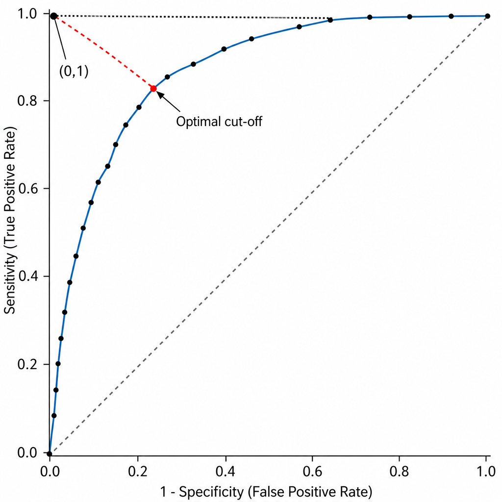
A clinician wants to select the single cut-off point on a diagnostic biomarker's ROC curve that minimizes the Euclidean distance to the upper-left corner (0,1), thereby simultaneously minimizing the false-negative rate and the false-positive rate. Which of the following best describes this optimal cut-off point selection criterion on the ROC curve?
A researcher wants to determine whether there is an association between CRP values and the risk of MI or cancer. Four relative risk (RR) values were plotted $(0.5,1.5,1.7,1.8)$ with respect to CRP levels. What conclusion can be drawn?
A researcher wants to study the carcinogenic effects of a food additive. From the literature, he finds that 7 different types of cancers have been linked to the consumption of this food additive. He wants to study all 7 possible outcomes. He conducts interviews with people who consume food containing these additives and people who do not. He then follows both groups for several years to see if they develop any of these 7 cancers or any other health outcomes. Which of the following study models best represents this study?
A 52-year-old man comes to the physician for a follow-up examination 1 year after an uncomplicated liver transplantation. He feels well but wants to know how long he can expect his donor graft to function. The physician informs him that the odds of graft survival are 90% at 1 year, 78% at 5 years, and 64% at 10 years. At this time, given that the graft has already survived 1 year, the probability of the patient's graft surviving to 10 years after transplantation is closest to which of the following?
The study is performed to examine the association between type 2 diabetes mellitus (DM2) and Alzheimer's disease (AD). Group of 250 subjects diagnosed with DM2 and a matched group of 250 subjects without DM2 are enrolled. Each subject is monitored regularly over their lifetime for the development of symptoms of dementia or mild cognitive impairment. If symptoms are present, an autopsy is performed after the patient's death to confirm the diagnosis of AD. Which of the following is most correct regarding this study?
A population is studied for risk factors associated with testicular cancer. Alcohol exposure, smoking, dietary factors, social support, and environmental exposure are all assessed. The researchers are interested in the incidence and prevalence of the disease in addition to other outcomes. Which pair of studies would best assess the 1. incidence and 2. prevalence?
A researcher is designing an experiment to examine the toxicity of a new chemotherapeutic agent in mice. She splits the mice into 2 groups, one of which she exposes to daily injections of the drug for 1 week. The other group is not exposed to any intervention. Both groups are otherwise raised in the same conditions with the same diet. One month later, she sacrifices the mice to check for dilated cardiomyopathy. In total, 52 mice were exposed to the drug, and 50 were not exposed. Out of the exposed group, 13 were found to have dilated cardiomyopathy on necropsy. In the unexposed group, 1 mouse was found to have dilated cardiomyopathy. Which of the following is the relative risk of developing cardiomyopathy with this drug?
A research group designs a study to investigate the epidemiology of syphilis in the United States. After a review of medical records, the investigators identify patients who are active cocaine users but did not have a history of syphilis as of one year ago. Another group of similar patients with no history of cocaine use or syphilis infection is also identified. The investigators examine the medical charts to determine whether the group of patients who are actively using cocaine was more likely to have developed syphilis over a 6-month period. The investigators ultimately found that the rate of syphilis was 30% higher in patients with active cocaine use compared to patients without cocaine use. This study is best described as which of the following?
A cohort study was conducted to investigate the impact of post-traumatic stress disorder (PTSD) on asthma symptoms in a group of firefighters who worked at Ground Zero during the September 11, 2001 terrorist attacks in New York City and developed asthma in the attack's aftermath. The study compared patients who had PTSD with those who did not have PTSD in order to determine if PTSD is associated with worse asthma control. During a follow-up period of 12 months, the researchers found that patients with PTSD had a greater number of hospitalizations for asthma exacerbations (RR = 2.0, 95% confidence interval = 1.4–2.5) after adjusting for medical comorbidities, psychiatric comorbidities other than PTSD, and sociodemographic variables. Results are shown: ≥ 1 asthma exacerbation No asthma exacerbations PTSD 80 80 No PTSD 50 150 Based on these results, what proportion of asthma hospitalizations in patients with PTSD could be attributed to PTSD?
A prospective cohort study was conducted to assess the relationship between LDL and the incidence of heart disease. The patients were selected at random. Results showed a 10-year relative risk (RR) of 3.0 for people with elevated LDL levels compared to individuals with normal LDL levels. The p-value was 0.04 with a 95% confidence interval of 2.0-4.0. According to the study results, what percent of heart disease in these patients can be attributed to elevated LDL?
Practice by Chapter
Prospective cohort design
Practice Questions
Retrospective cohort design
Practice Questions
Exposure assessment
Practice Questions
Follow-up methods
Practice Questions
Loss to follow-up handling
Practice Questions
Time-to-event analysis
Practice Questions
Survival curves
Practice Questions
Cox proportional hazards model
Practice Questions
Competing risks
Practice Questions
Nested case-control studies
Practice Questions
Case-cohort studies
Practice Questions
Historical cohorts
Practice Questions
Strengths and limitations of cohort studies
Practice Questions
Want unlimited practice?
Get full access to all questions, explanations, and performance tracking.
Scan to download app